Bulk RNAseq report
Gianluca Alessio Mariani
29 October, 2025
Last updated: 2025-10-29
Checks: 7 0
Knit directory: frascolla_chemoresistance/
This reproducible R Markdown analysis was created with workflowr (version 1.7.2). The Checks tab describes the reproducibility checks that were applied when the results were created. The Past versions tab lists the development history.
Great! Since the R Markdown file has been committed to the Git repository, you know the exact version of the code that produced these results.
Great job! The global environment was empty. Objects defined in the global environment can affect the analysis in your R Markdown file in unknown ways. For reproduciblity it’s best to always run the code in an empty environment.
The command set.seed(20250522) was run prior to running
the code in the R Markdown file. Setting a seed ensures that any results
that rely on randomness, e.g. subsampling or permutations, are
reproducible.
Great job! Recording the operating system, R version, and package versions is critical for reproducibility.
Nice! There were no cached chunks for this analysis, so you can be confident that you successfully produced the results during this run.
Great job! Using relative paths to the files within your workflowr project makes it easier to run your code on other machines.
Great! You are using Git for version control. Tracking code development and connecting the code version to the results is critical for reproducibility.
The results in this page were generated with repository version b3bf26c. See the Past versions tab to see a history of the changes made to the R Markdown and HTML files.
Note that you need to be careful to ensure that all relevant files for
the analysis have been committed to Git prior to generating the results
(you can use wflow_publish or
wflow_git_commit). workflowr only checks the R Markdown
file, but you know if there are other scripts or data files that it
depends on. Below is the status of the Git repository when the results
were generated:
Untracked files:
    Untracked:  .DS_Store
    Untracked:  analysis/01_baseline_analysis_ex.Rmd
    Untracked:  analysis/_expression_barplot.Rmd
    Untracked:  data/251015_genelist_frascolla.csv
    Untracked:  data/RNAseq_analysis.xlsx
    Untracked:  data/RNAseq_analysis_gene_lists.xlsx
    Untracked:  data/UNIQUELIST_shIFI6_vs_shIFI6.csv
    Untracked:  data/UNIQUELIST_shIFI6_vs_shSCR.csv
    Untracked:  data/apoptosis_gene_list.csv
    Untracked:  data/apoptosis_gene_list.xlsx
    Untracked:  data/sample_list_variables.csv
    Untracked:  data/samples_info_sh1plus2_vs_scr.tsv
    Untracked:  data/samples_list.csv
    Untracked:  data/shIFI6 Day 5 vs Day 0.csv
    Untracked:  data/shIFI6Day 3 vs shSCRDay 0.csv
    Untracked:  data/shIFI6Day 4 vs Day 0.csv
    Untracked:  data/shIFI6Day 4 vs shSCRDay 0.csv
    Untracked:  data/shIFI6Day 5 vs shSCRDay 0.csv
    Untracked:  data/shIFI6Day3 vs Day0.csv
    Untracked:  data/shIFI6_vs_shIFI6_FINAL.csv
    Untracked:  data/shIFI6_vs_shSCR_FINAL.csv
    Untracked:  output/deg_shIFI6_Day0_vs_shSCR_Day0.tsv
    Untracked:  output/deg_shIFI6_Day0_vs_shSCR_Day4.tsv
    Untracked:  output/deg_shIFI6_Day1_vs_shSCR_Day0.tsv
    Untracked:  output/deg_shIFI6_Day2_vs_shSCR_Day0.tsv
    Untracked:  output/deg_shIFI6_Day3_vs_shSCR_Day0.tsv
    Untracked:  output/deg_shIFI6_Day4_vs_shSCR_Day0.tsv
    Untracked:  output/deg_shIFI6_Day5_vs_shSCR_Day0.tsv
    Untracked:  output/deg_shSCR_Day2_vs_shSCR_Day0.tsv
    Untracked:  output/deg_shSCR_Day3_vs_shSCR_Day0.tsv
    Untracked:  output/deg_shSCR_Day4_vs_shSCR_Day0.tsv
    Untracked:  src/a
    Untracked:  src/genes2filter_ensemblid.csv
    Untracked:  src/genes2filter_symbol.csv
    Untracked:  src/h.all.v2025.1.Hs.symbols.gmt

Unstaged changes:
    Modified:   analysis/06_de_ifi6_day0_scr_day4.Rmd
    Modified:   output/deg_shIFI6_1_Day1_vs_shSCR_Day1.tsv
    Modified:   output/deg_shIFI6_1_Day2_vs_shSCR_Day2.tsv
    Modified:   output/deg_shIFI6_1_Day3_vs_shSCR_Day3.tsv
    Modified:   output/deg_shIFI6_1_Day4_vs_shSCR_Day4.tsv
    Modified:   output/deg_shIFI6_1_Day5_vs_shSCR_Day5.tsv
    Modified:   output/deg_shIFI6_2_Day1_vs_shSCR_Day1.tsv
    Modified:   output/deg_shIFI6_2_Day2_vs_shSCR_Day2.tsv
    Modified:   output/deg_shIFI6_2_Day3_vs_shSCR_Day3.tsv
    Modified:   output/deg_shIFI6_2_Day4_vs_shSCR_Day4.tsv
    Modified:   output/deg_shIFI6_2_Day5_vs_shSCR_Day5.tsv
    Modified:   output/deg_shIFI6_Day1_vs_shIFI6_Day0.tsv
    Modified:   output/deg_shIFI6_Day1_vs_shSCR_Day1.tsv
    Modified:   output/deg_shIFI6_Day2_vs_shIFI6_Day0.tsv
    Modified:   output/deg_shIFI6_Day2_vs_shSCR_Day2.tsv
    Modified:   output/deg_shIFI6_Day3_vs_shIFI6_Day0.tsv
    Modified:   output/deg_shIFI6_Day3_vs_shSCR_Day3.tsv
    Modified:   output/deg_shIFI6_Day4_vs_shIFI6_Day0.tsv
    Modified:   output/deg_shIFI6_Day4_vs_shSCR_Day4.tsv
    Modified:   output/deg_shIFI6_Day5_vs_shIFI6_Day0.tsv
    Modified:   output/deg_shIFI6_Day5_vs_shSCR_Day5.tsv
    Modified:   output/deg_shSCR_Day1_vs_shSCR_Day0.tsv
    Modified:   output/deg_shSCR_Day5_vs_shSCR_Day0.tsv
    Modified:   src/__utils_rna_seq_functions.R
Note that any generated files, e.g. HTML, png, CSS, etc., are not included in this status report because it is ok for generated content to have uncommitted changes.
These are the previous versions of the repository in which changes were
made to the R Markdown (analysis/01_baseline_analysis.Rmd)
and HTML (docs/01_baseline_analysis.html) files. If you’ve
configured a remote Git repository (see ?wflow_git_remote),
click on the hyperlinks in the table below to view the files as they
were in that past version.
| File | Version | Author | Date | Message |
|---|---|---|---|---|
| Rmd | b3bf26c | Mariani_Gianluca_Alessio | 2025-10-29 | Added Apoptosis heatmaps |
| html | 078db00 | Mariani_Gianluca_Alessio | 2025-10-20 | Build site. |
| Rmd | 4c274d4 | Mariani_Gianluca_Alessio | 2025-10-20 | Added gene expression heatmaps |
| html | 802e424 | Mariani_Gianluca_Alessio | 2025-09-29 | Build site. |
| Rmd | 52502b5 | Mariani_Gianluca_Alessio | 2025-09-29 | Added enrichment score for every pathway in the GSEA, added GO and HALLMARK terms for every gene in the genetables |
| html | 5b1051e | Mariani_Gianluca_Alessio | 2025-09-26 | Build site. |
| Rmd | 96c88b4 | Mariani_Gianluca_Alessio | 2025-09-26 | Added 4 average selected gene expression barplots |
| html | 11f3d4d | Mariani_Gianluca_Alessio | 2025-07-16 | Build site. |
| html | 401e86f | Mariani_Gianluca_Alessio | 2025-07-15 | Build site. |
| Rmd | 57ef6f7 | Mariani_Gianluca_Alessio | 2025-07-15 | Redone analysis with ribosomal genes filter |
| html | a3e3ed2 | Yinxiu Zhan | 2025-07-10 | Build site. |
| Rmd | 13204d7 | Yinxiu Zhan | 2025-07-10 | Fix linking |
| html | 3cabe3c | Yinxiu Zhan | 2025-07-10 | Build site. |
| Rmd | 1e3bcd0 | Yinxiu Zhan | 2025-07-10 | Fix linking |
| Rmd | c0a0612 | Yinxiu Zhan | 2025-07-09 | :sparkles: Release first version |
knitr::opts_chunk$set(echo       = FALSE,
                      message    = FALSE,
                      warning    = FALSE,
                      cache      = FALSE,
                      autodep    = TRUE,
                      fig.align  = 'center',
                      fig.width  = 10,
                      fig.height = 8)
Introduction
FRASCOLLA AGGIUNGI
Overview of the analysis steps
- Quality control of raw data with FastQC
- Adapter and quality trimming with Trim Galore!
- Read alignment with STAR.
- Estimation of transcript and gene expression with Salmon.
- Differential gene expression analysis with DESeq2 (v1.49.1)
- Gene set enrichment analysis with ClusterProfiler (v4.17.0)
The steps from 1 to 4 have been performed using nf-core/rnaseq v3.18.0. This report includes analysis from step 5 and 6
Samples Datatable
Below we present the table containing all the samples analyzed in this report.
Each sample is described by:
sample: sample name defined a priori in the previous step of RNA seq analysis
condition_single: list of samples divided into groups based on the base condition and the time
condition_pooled: list of samples divided into groups based on the base condition and the time and grouping together the samples from the two shIFI6 conditions
base_condition: the baseline condition (control, knockdown, treated, etc…) irrespective of any other experimental variable/parameter
time: day after treatment
PCA Analysis
For the PCA (principal component analysis) and correlation analyses, gene expression data were normalized using the variance stabilizing transformation (VST) method implemented in DESeq2.
Below, we present the PCA performed on the complete set of samples. PCA was used to explore global variance in gene expression profiles across all samples.
The primary objectives of this analysis are to:
Assess sample quality
Determine whether samples cluster according to experimental conditions, suggesting biologically meaningful variation
Identify potential outliers
Detect batch effects or other sources of unwanted variation
By reducing the high-dimensional gene expression data into a few principal components, PCA provides a visual summary of the dataset’s structure.
Interpretation PCA Analysis and evaluation of batch effect
Un bordello
Correlation analysis
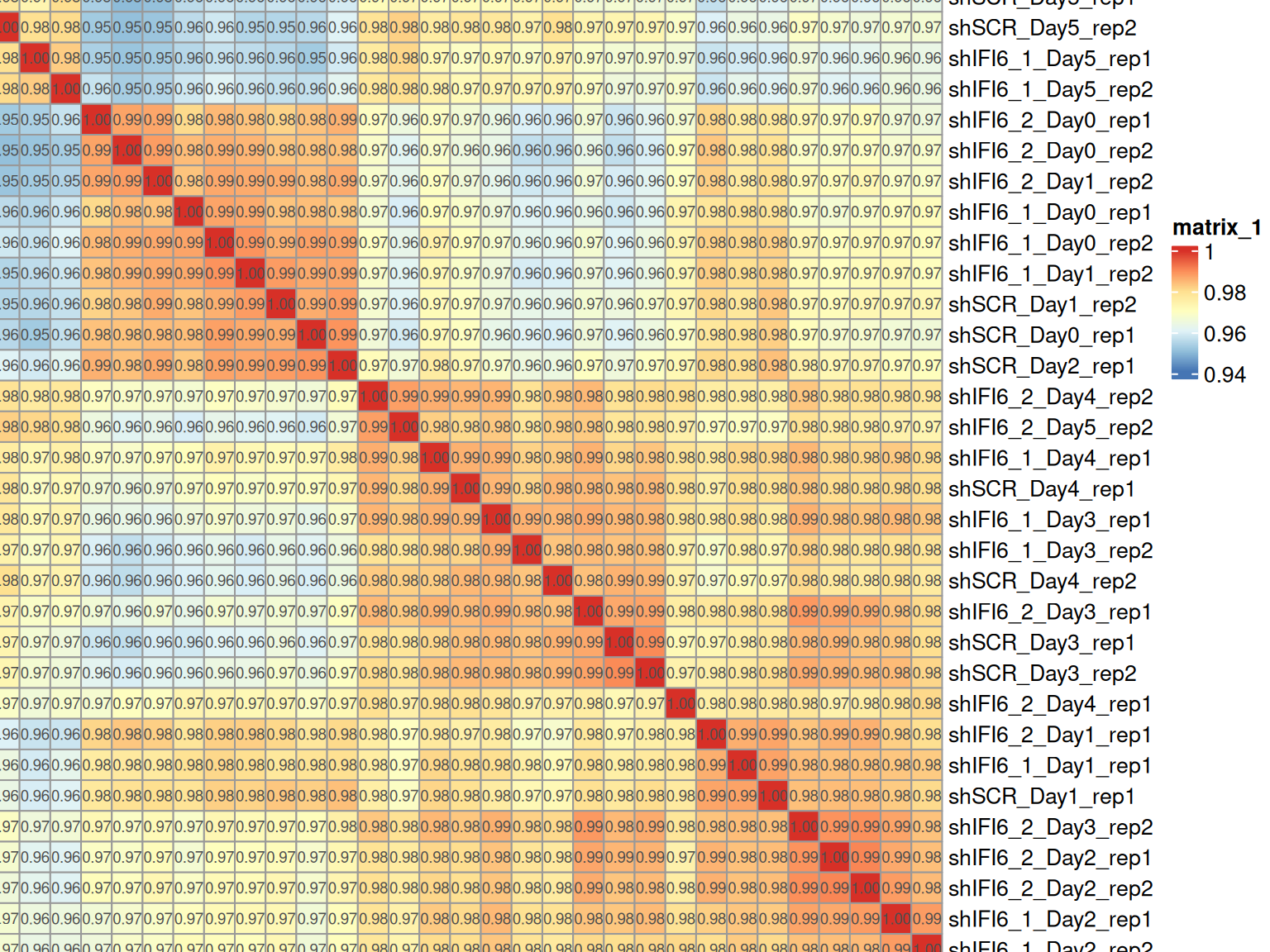
The Spearman correlation heatmap provides a global view of the similarity between gene expression profiles across all samples. We calculated the pairwise Spearman correlation coefficients between samples and visualized them in a heatmap. Rows and columns are hierarchically clustered based on these correlations to reveal patterns of similarity and potential groupings among samples.
Spearman Correlation: General Interpretation
High Correlation Values (> 0.98)
Between replicates of the same condition:
A very good quality signal
Indicates that replicates behave consistently
Suggests well-defined and reproducible biological conditions
Between different conditions:
May indicate minor transcriptional differences
Or poor separation due to contamination or mislabeling
Lower Correlation Values (< 0.95)
Between replicates of the same condition:
May suggest technical or biological issues:
Library prep/sequencing errors
Sample mix-up or mislabeling
Biological heterogeneity
In some cases, biological replicates may exhibit a certain degree of variability that cannot be entirely avoided. This is particularly true when samples are obtained from different individuals, such as patient-derived samples, even when all other experimental conditions are carefully controlled.
Therefore, lower correlation values between replicates should not be interpreted in a standardized way, but rather evaluated in the specific biological and experimental context of the study.
Between different conditions:
Expected when conditions are biologically distinct
If correlations are too similar to replicates, it may suggest:
Weak treatment effects
Few genes affected by the condition
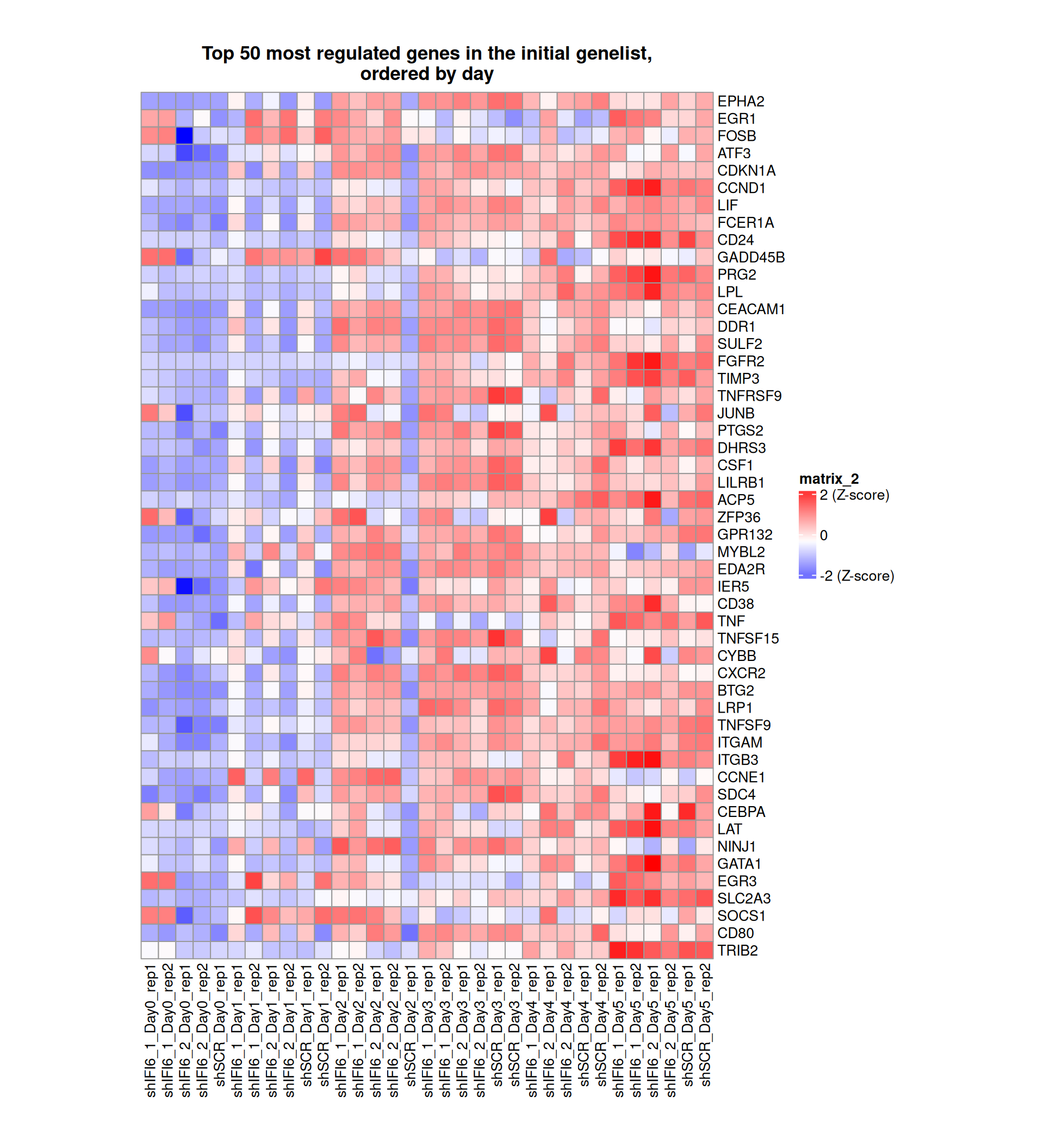
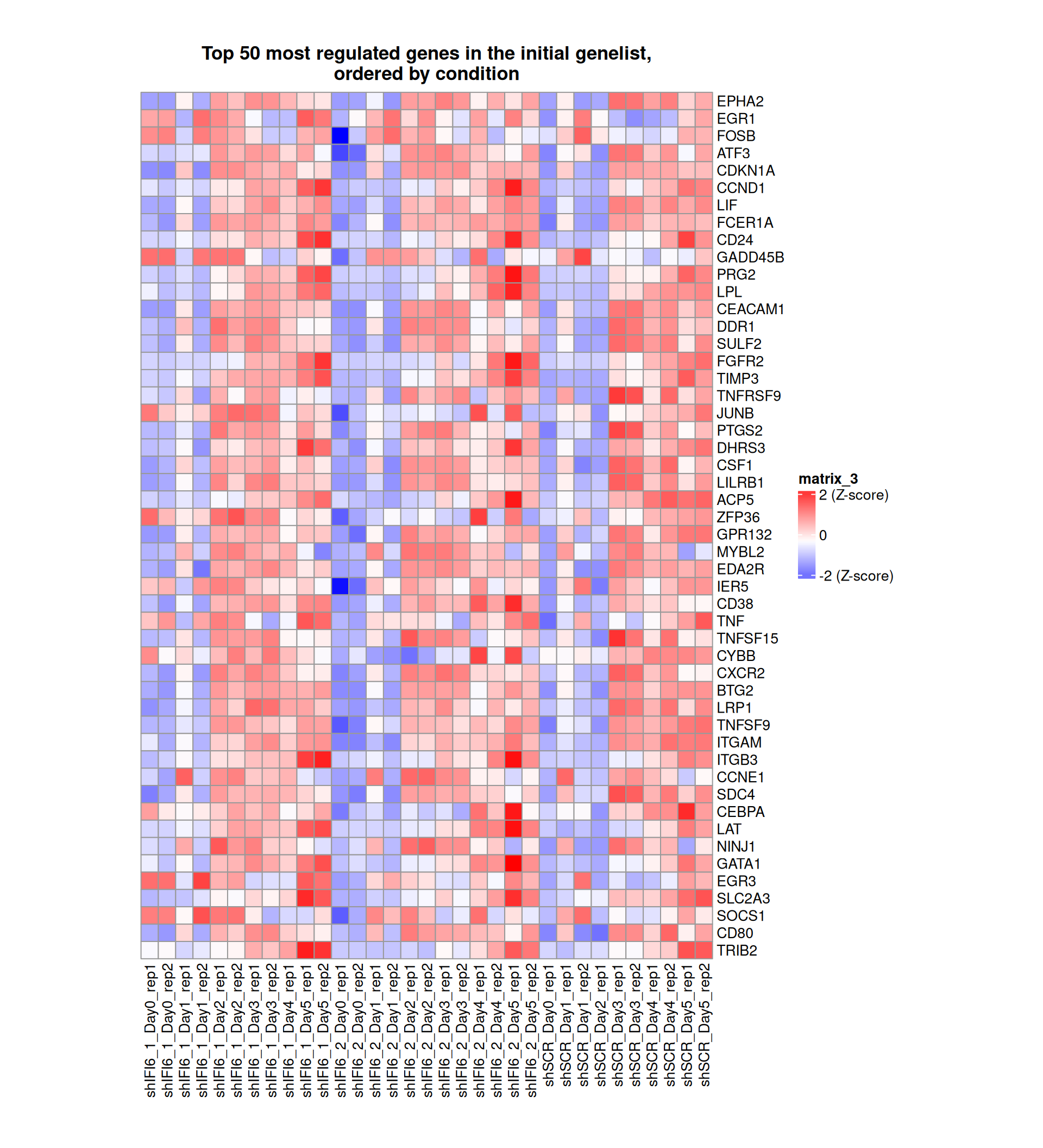
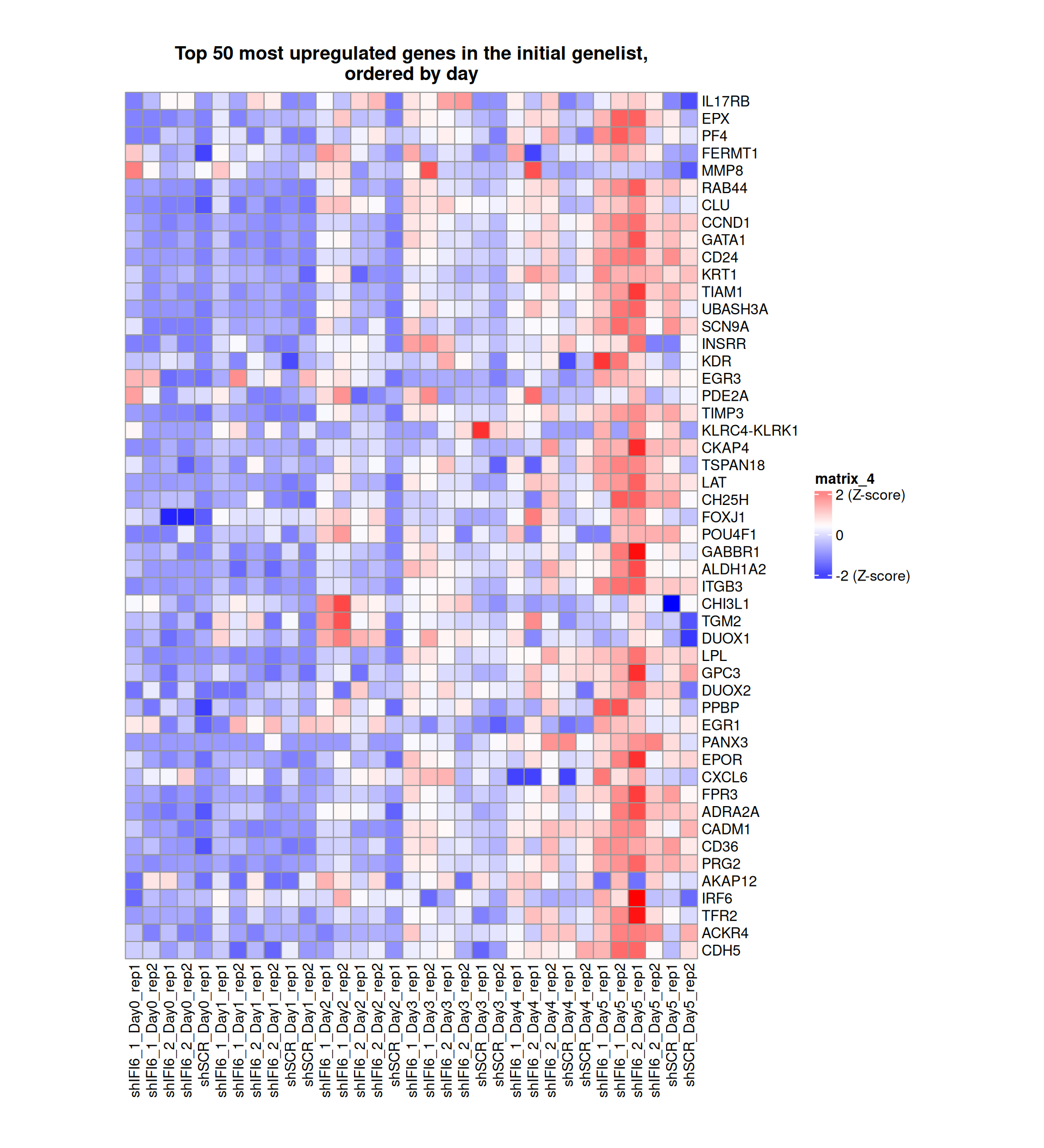
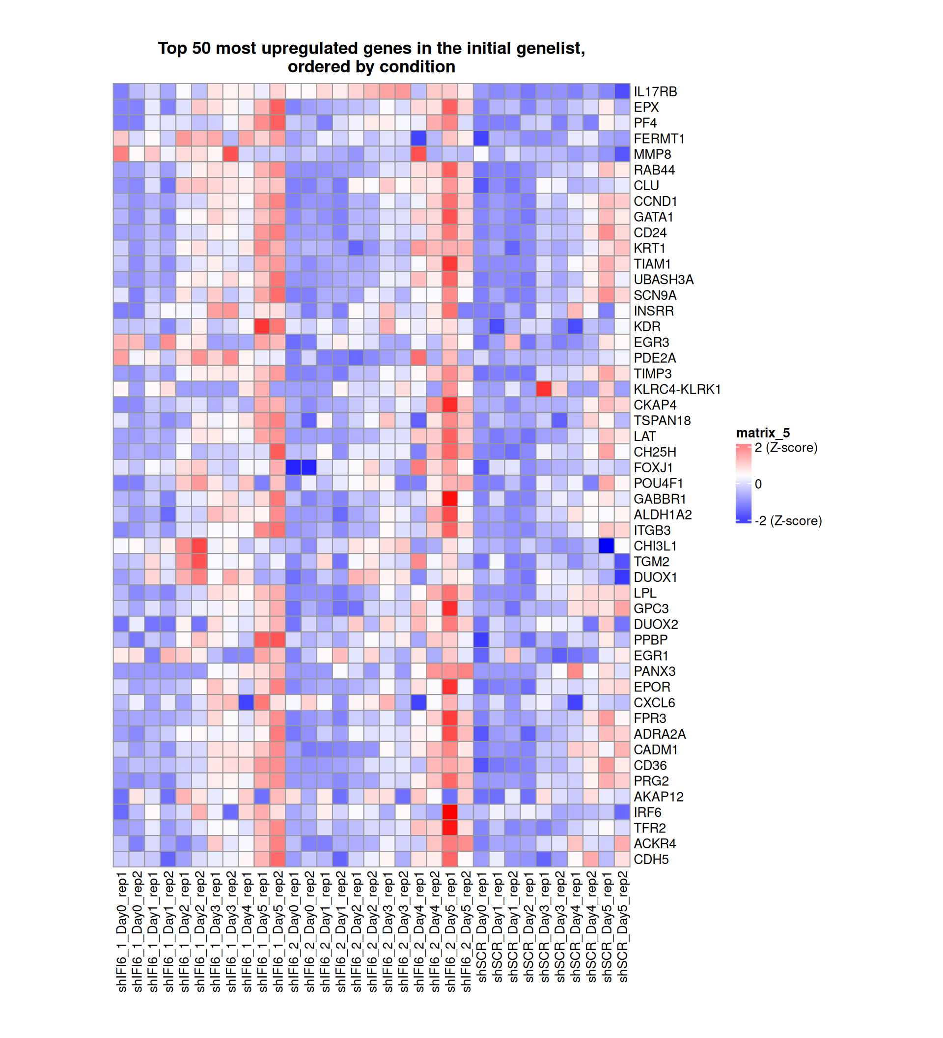
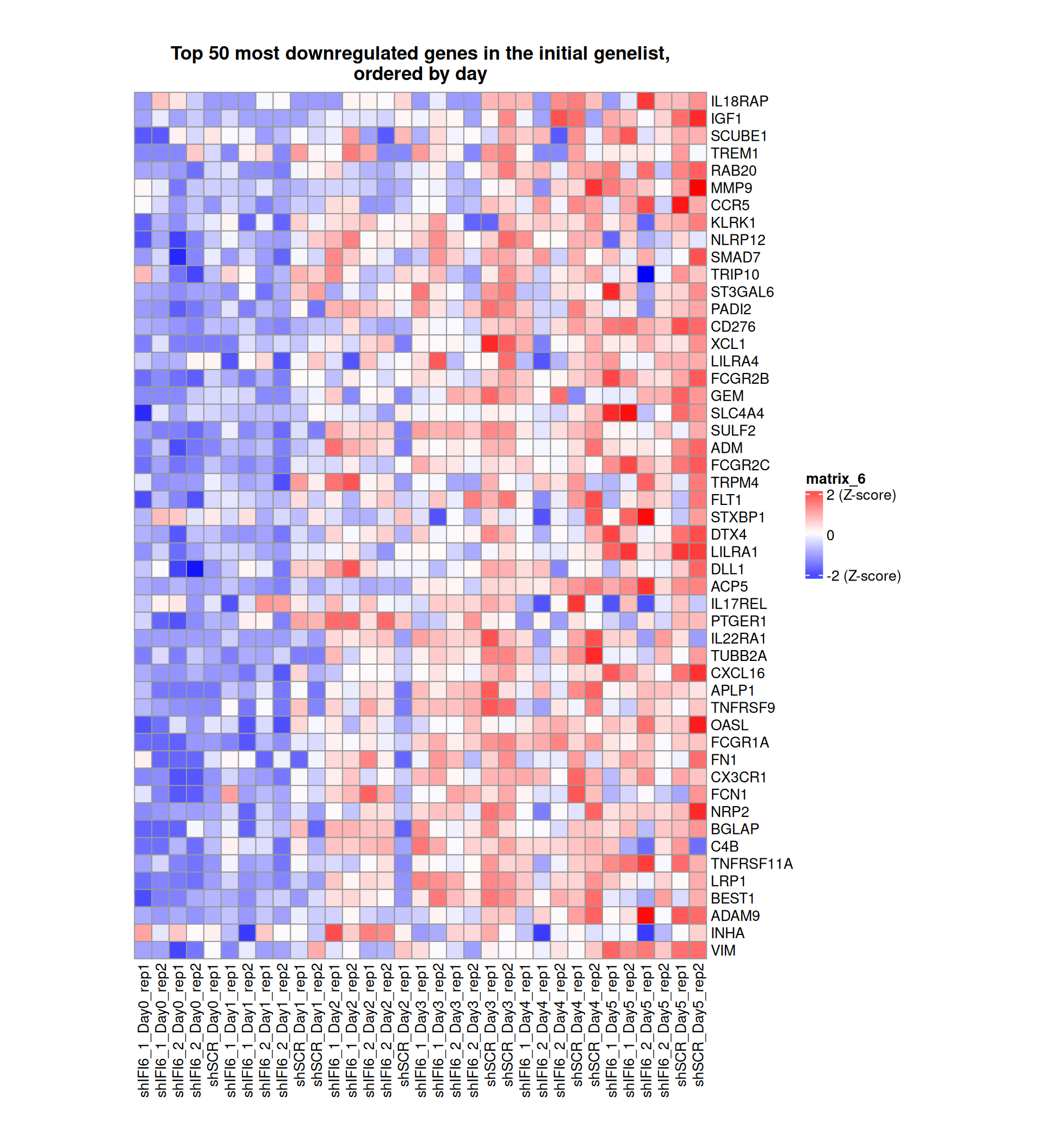
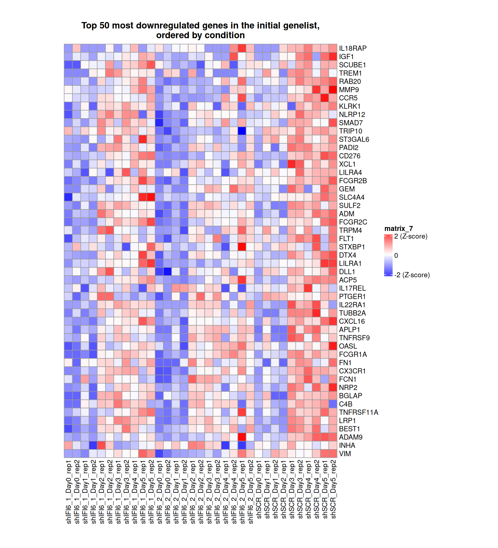
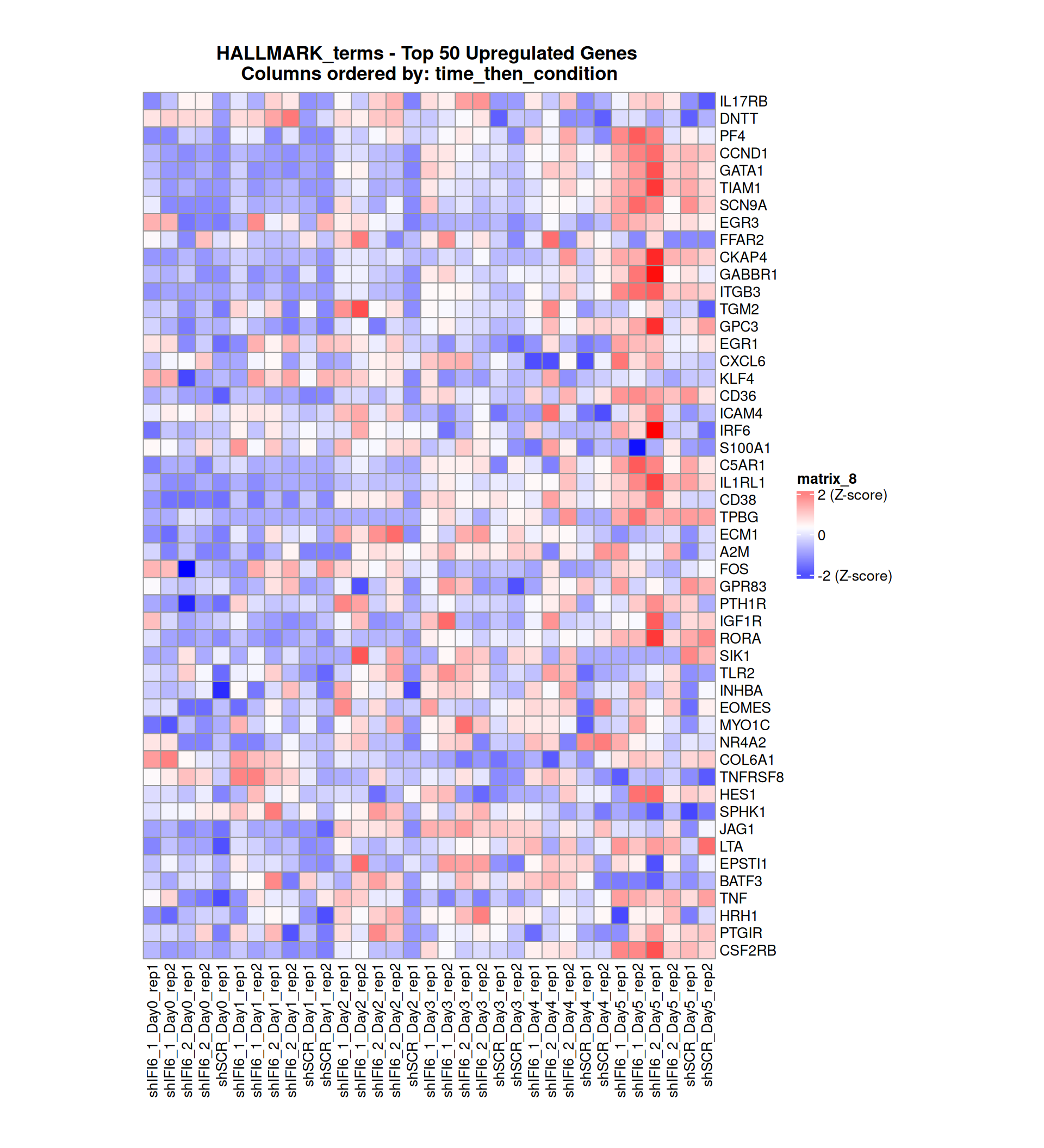
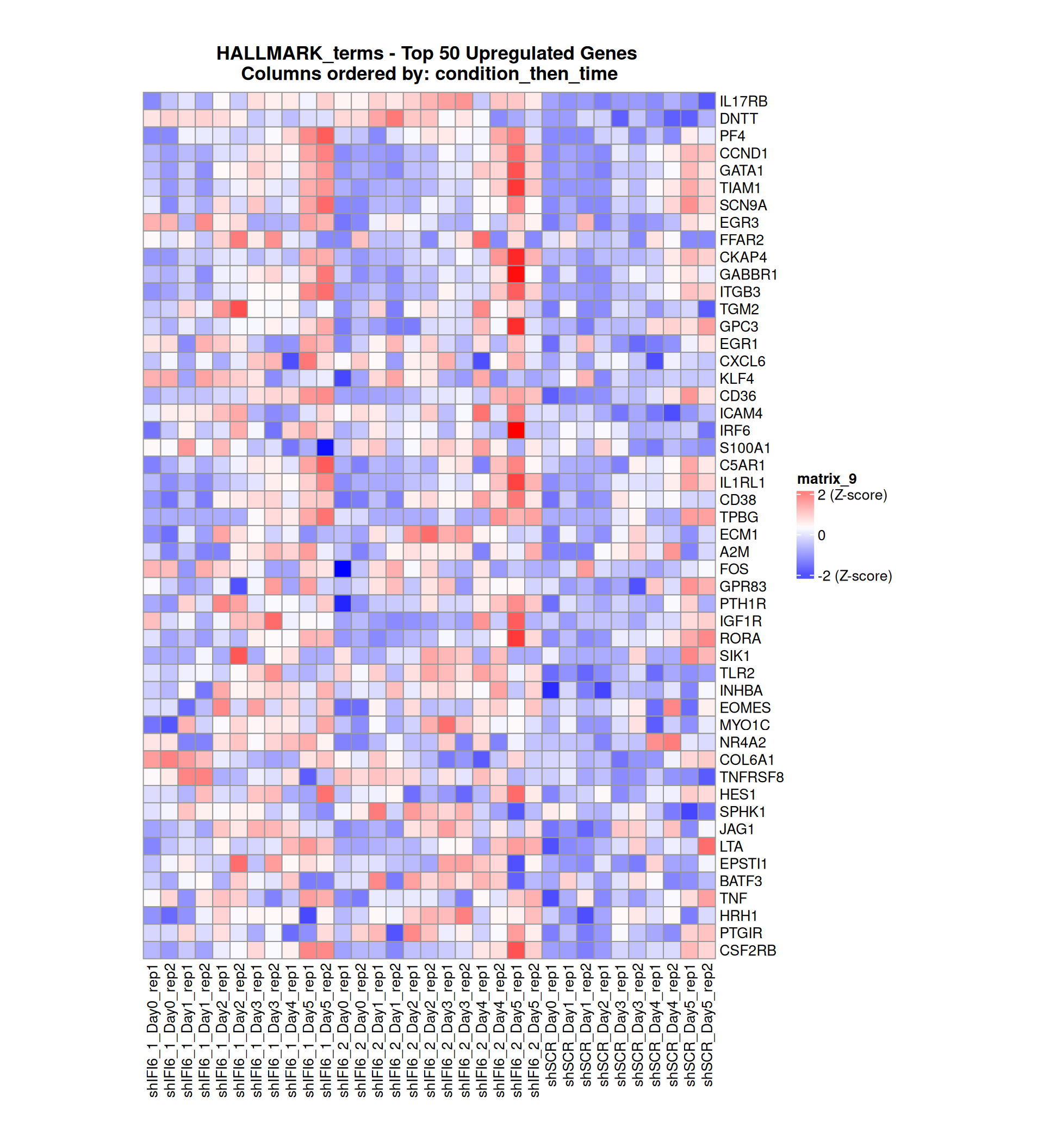
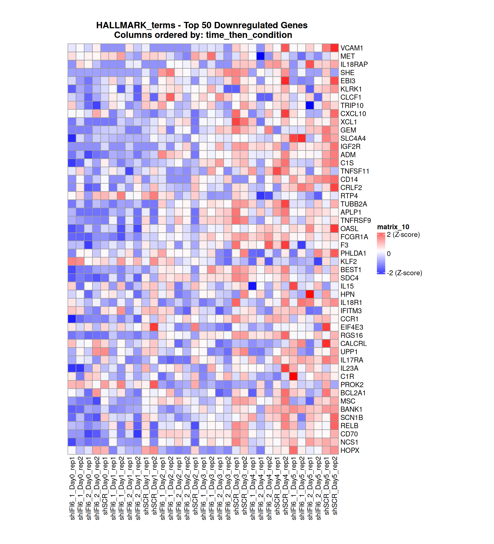
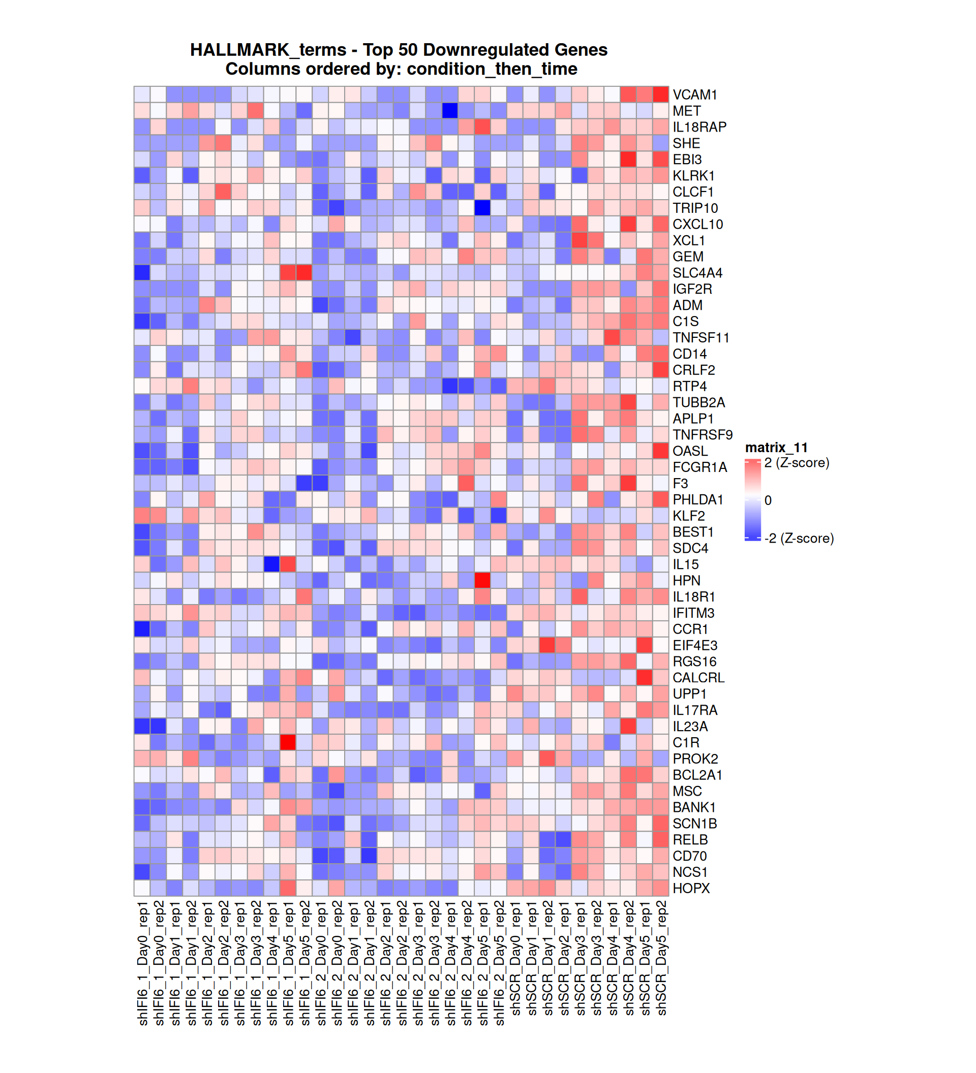
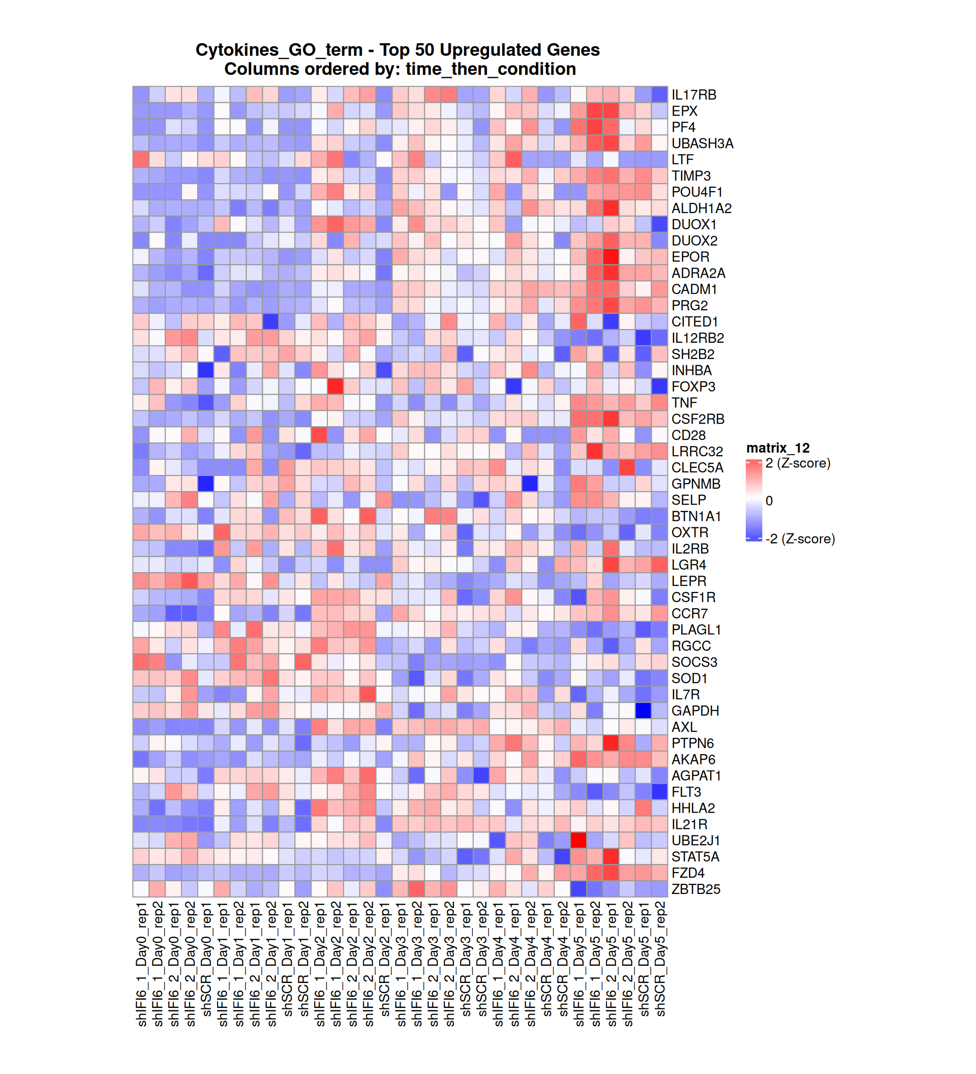
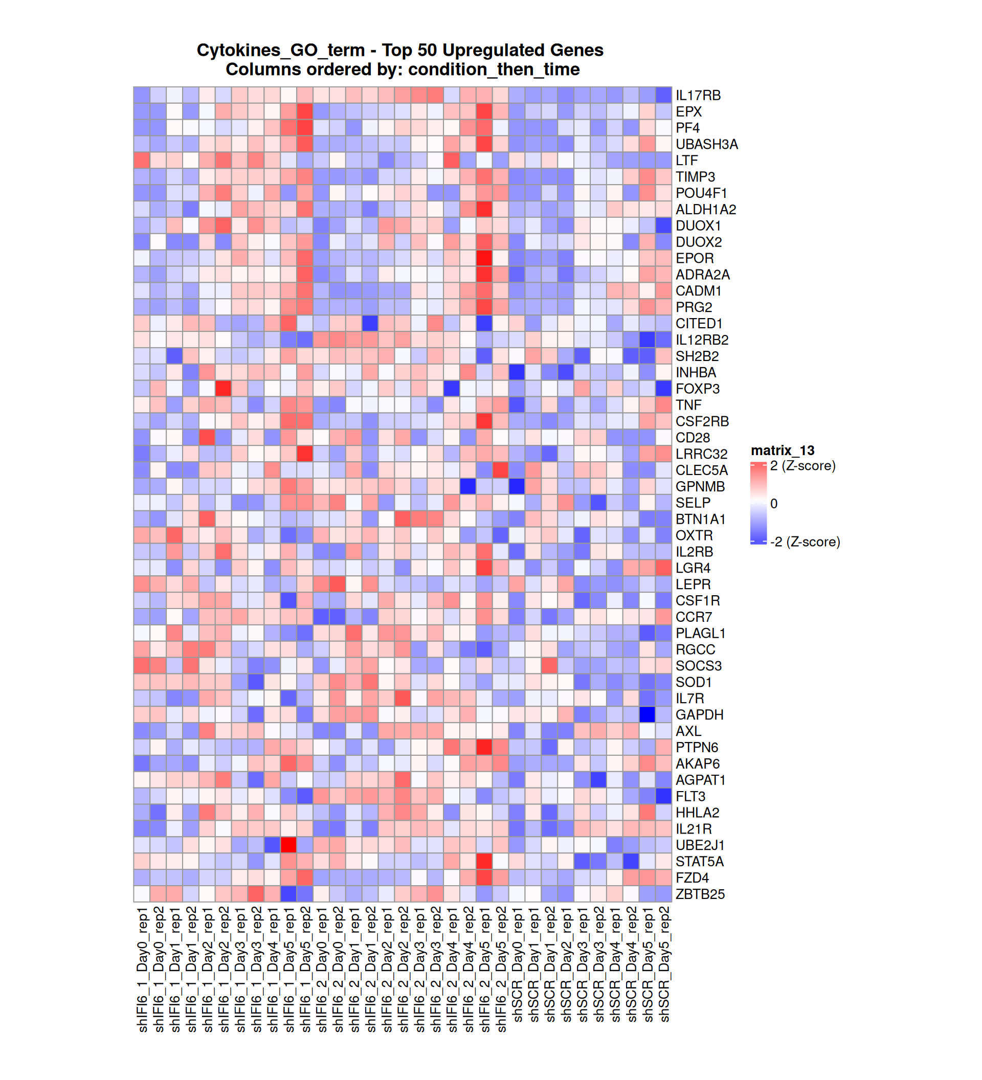
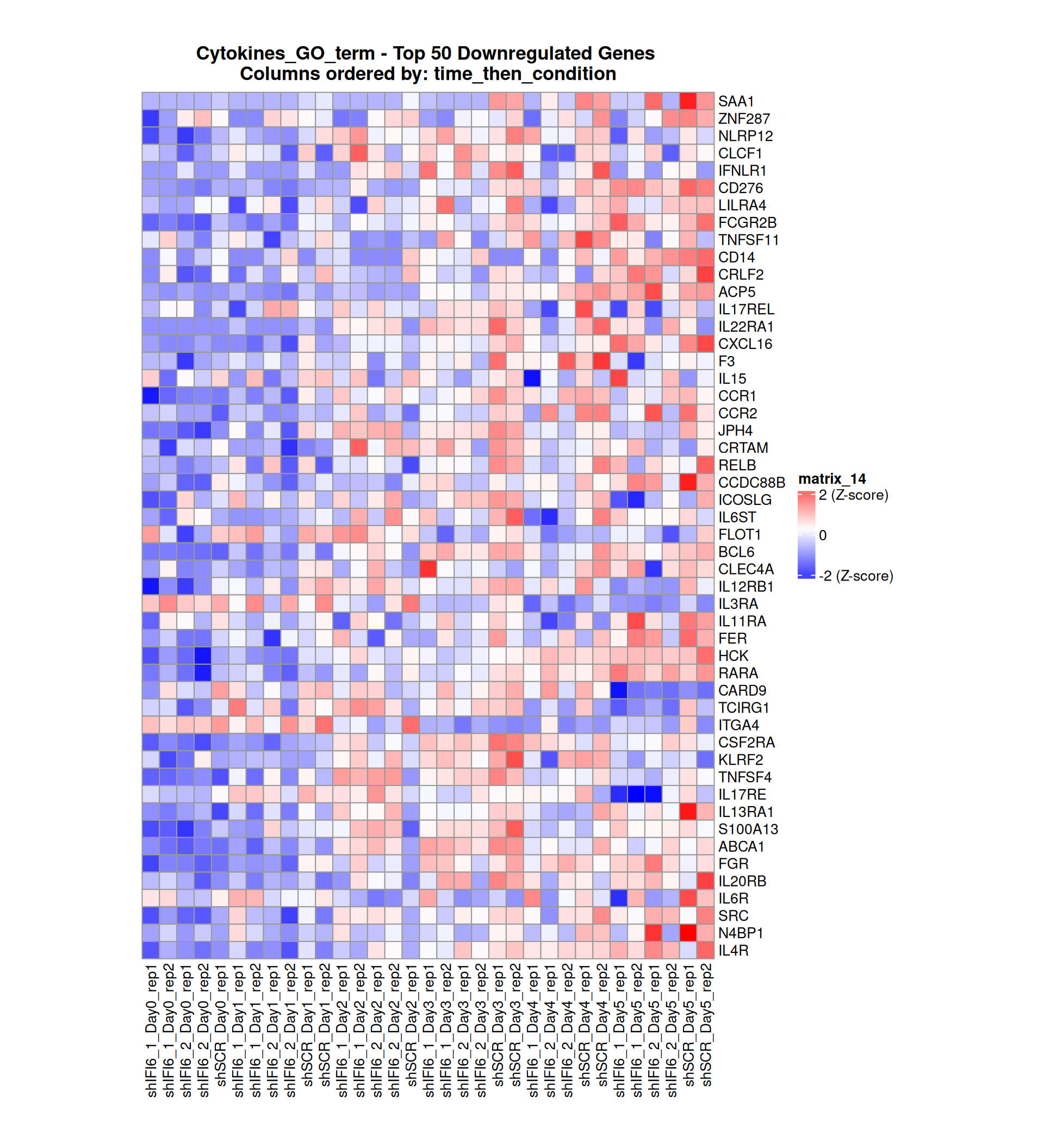
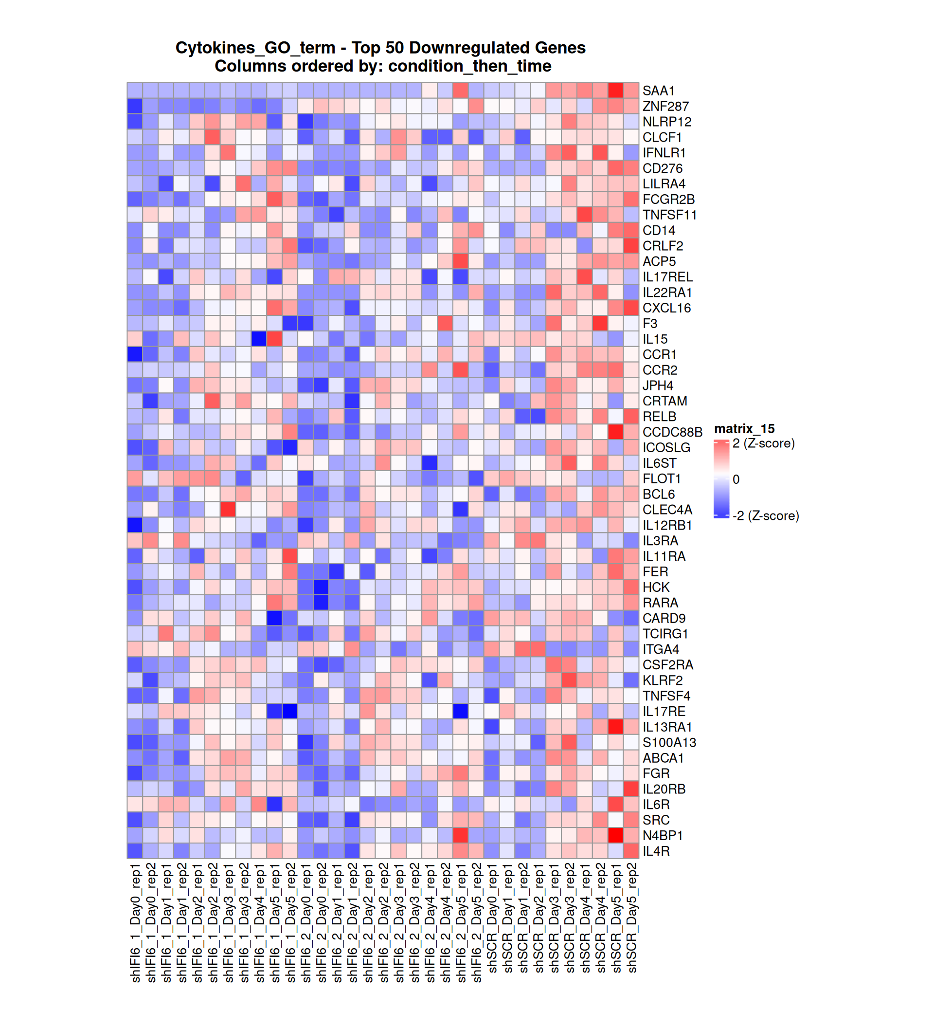
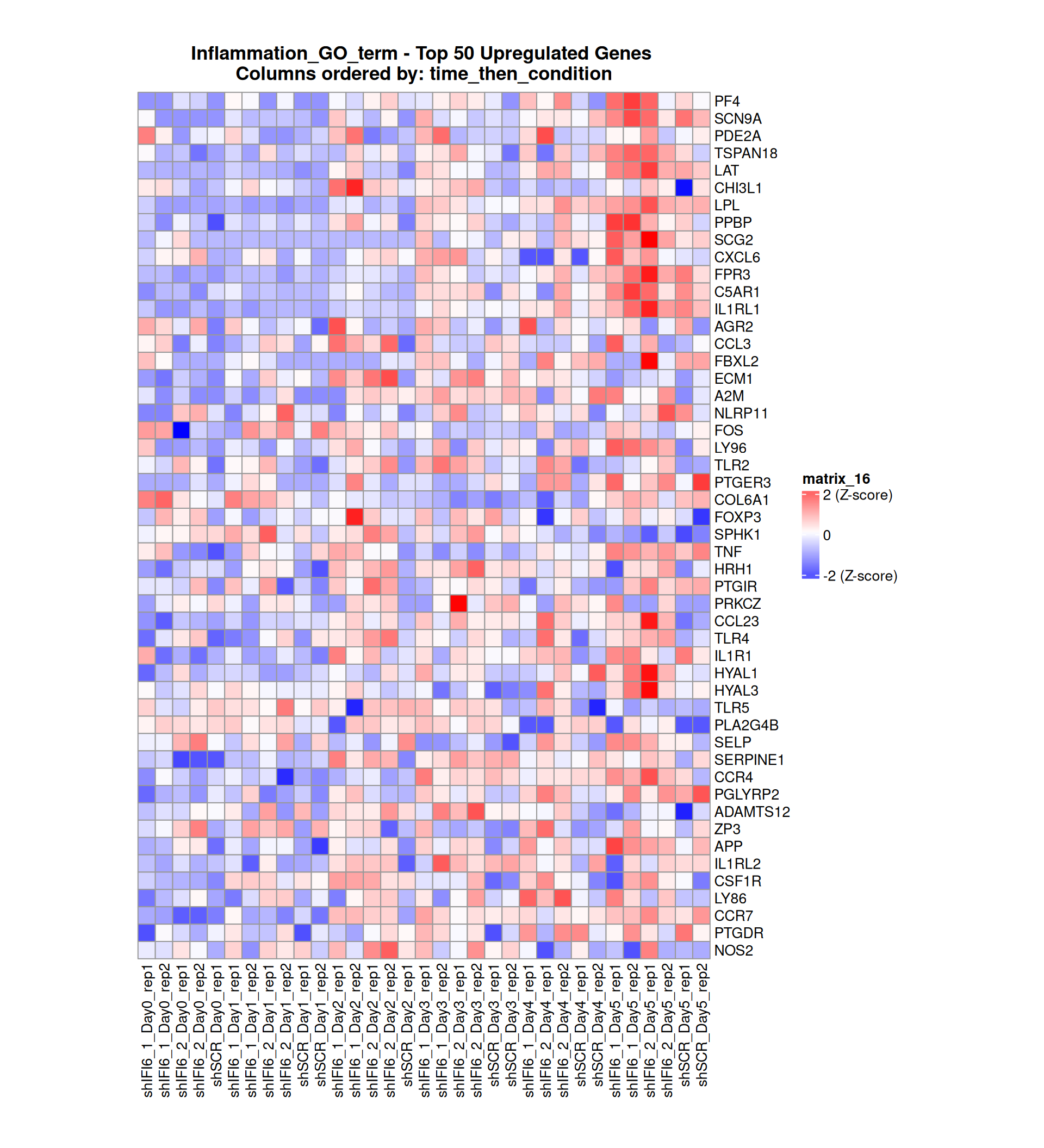
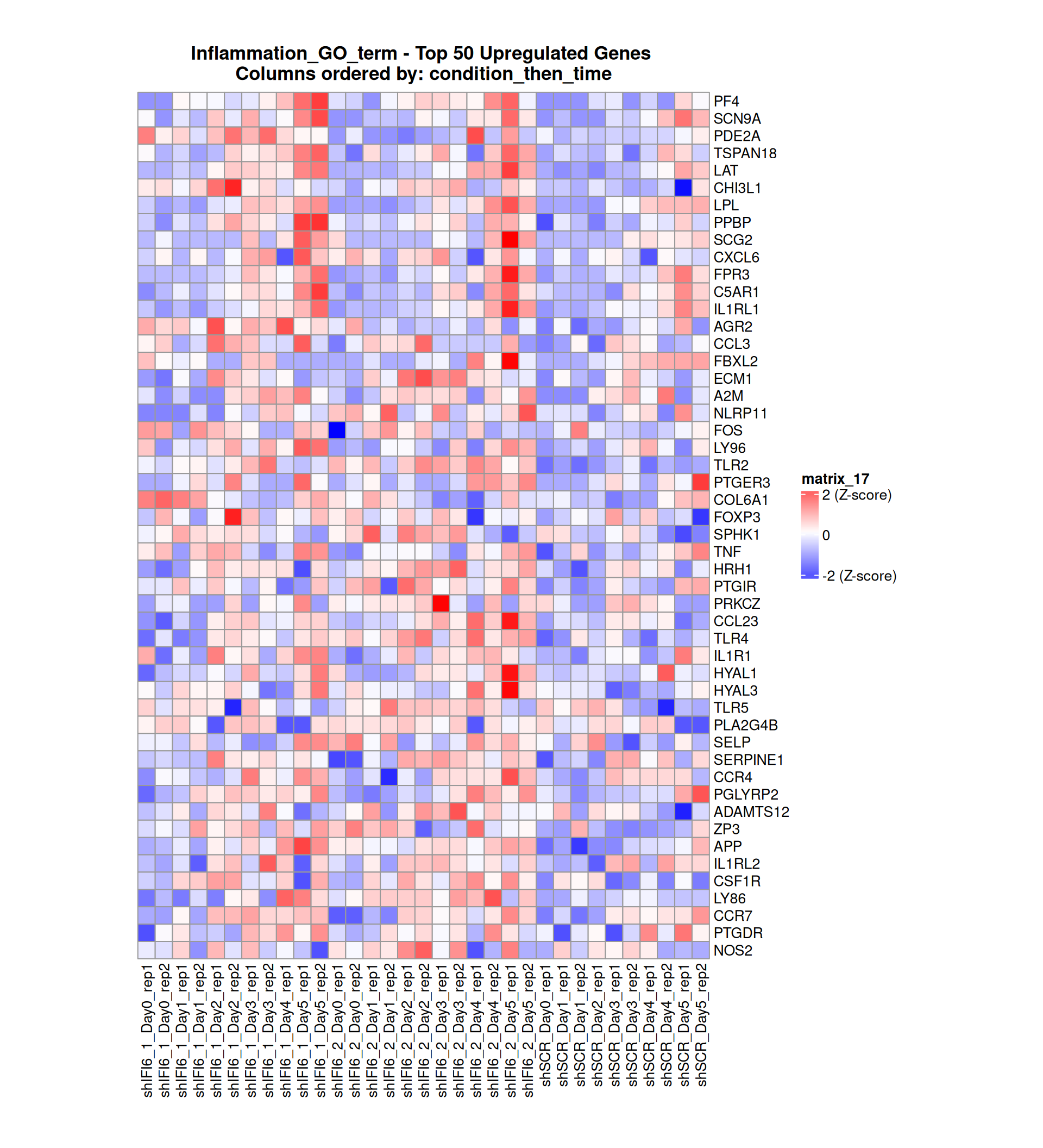
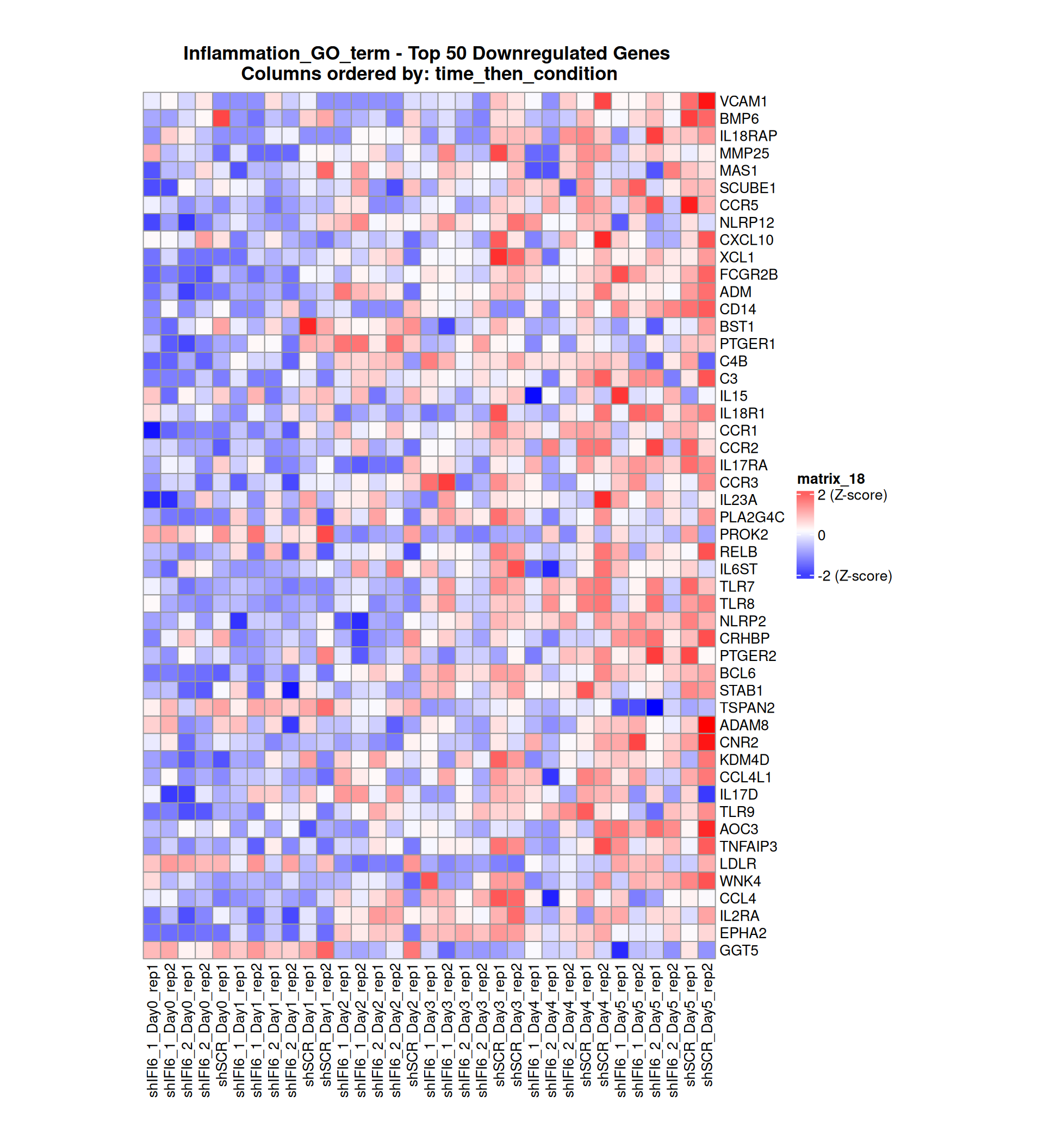
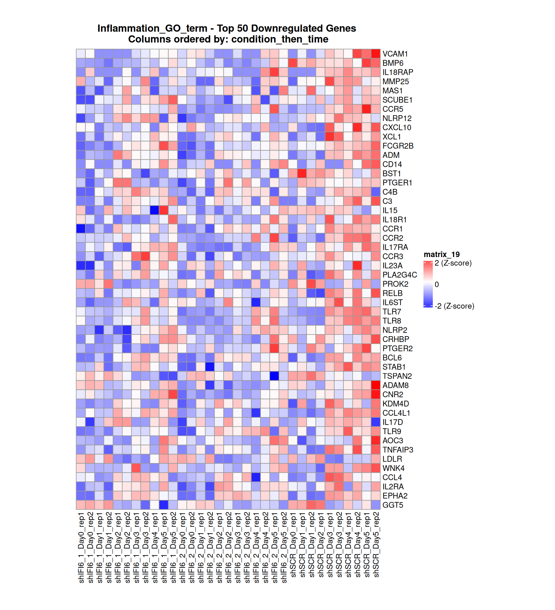
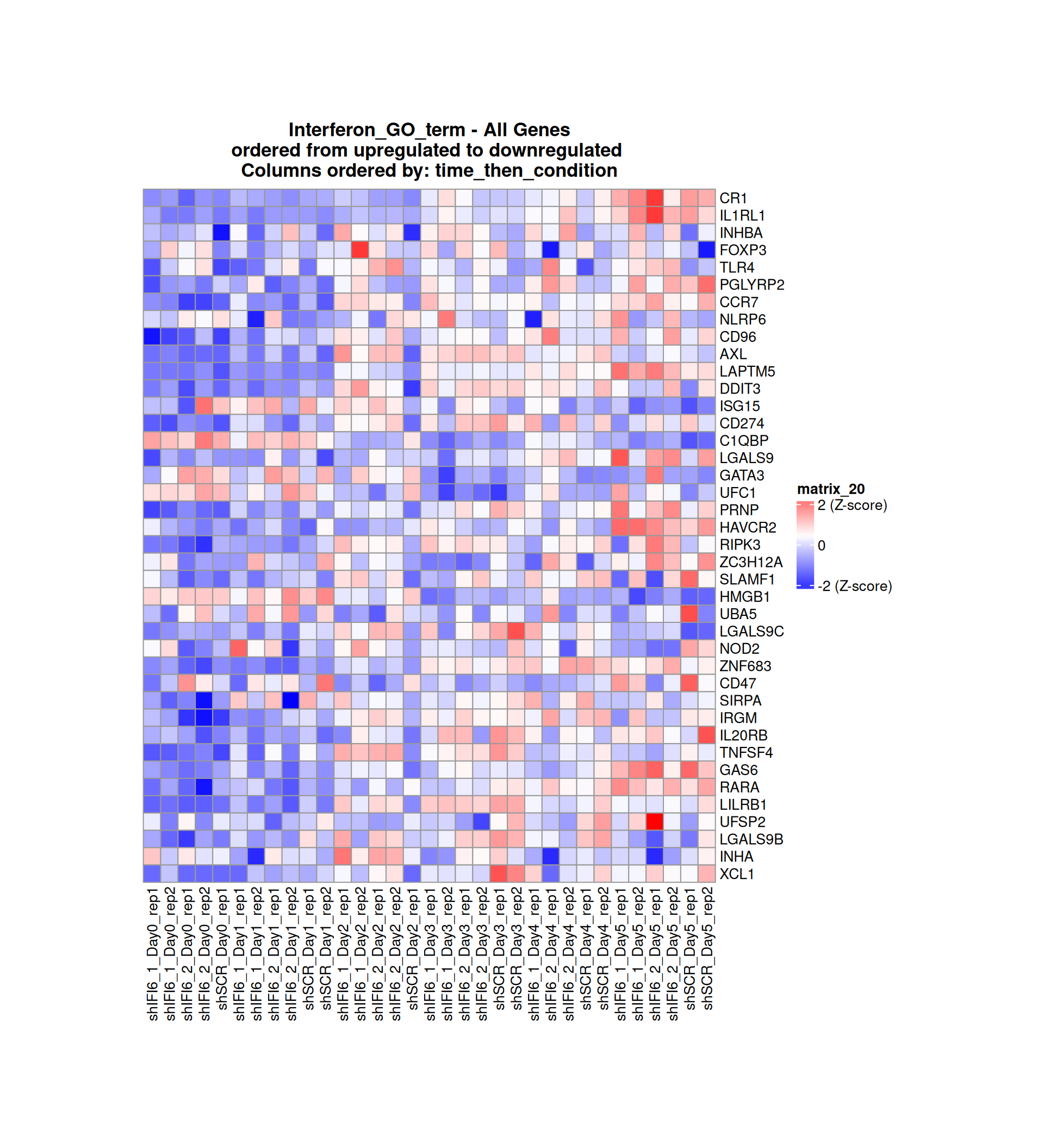
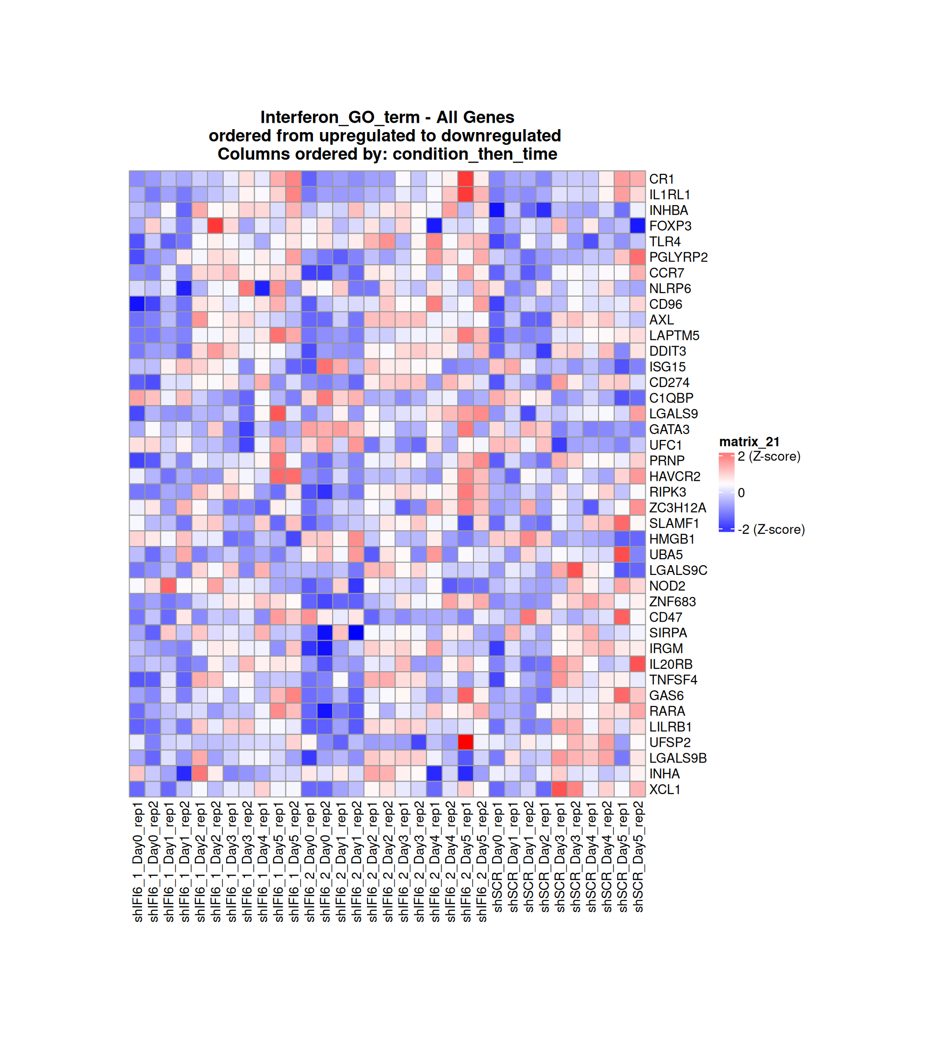
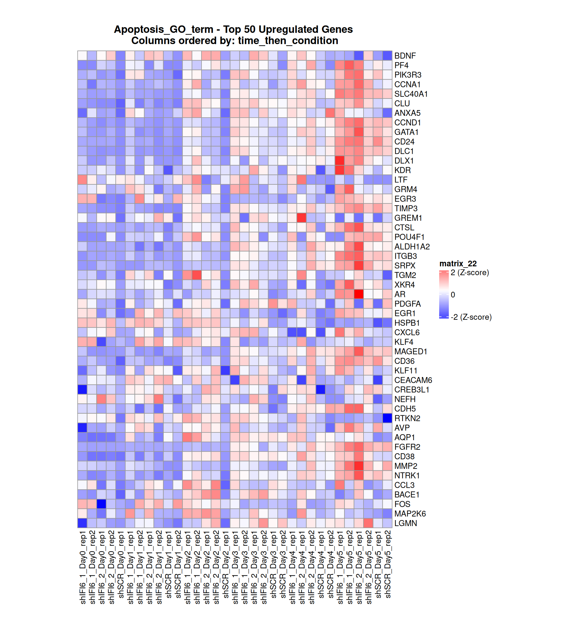
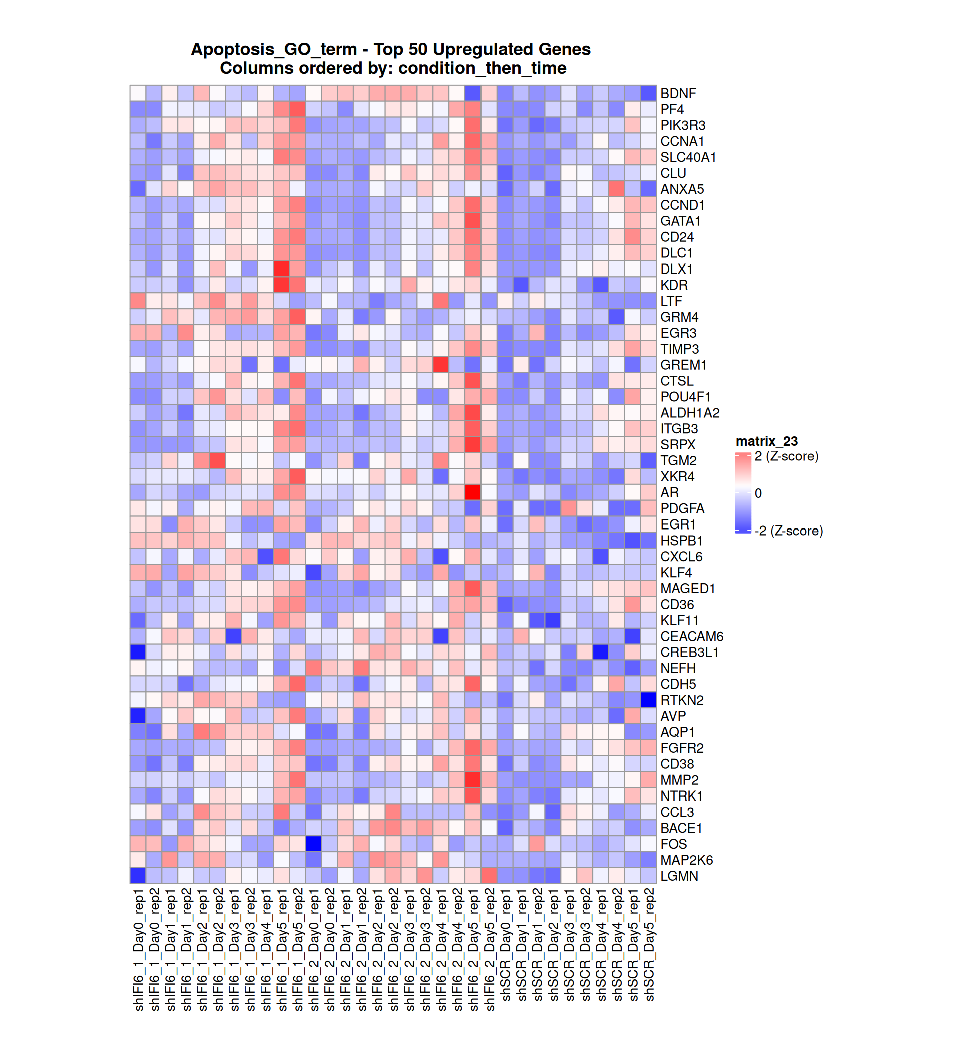
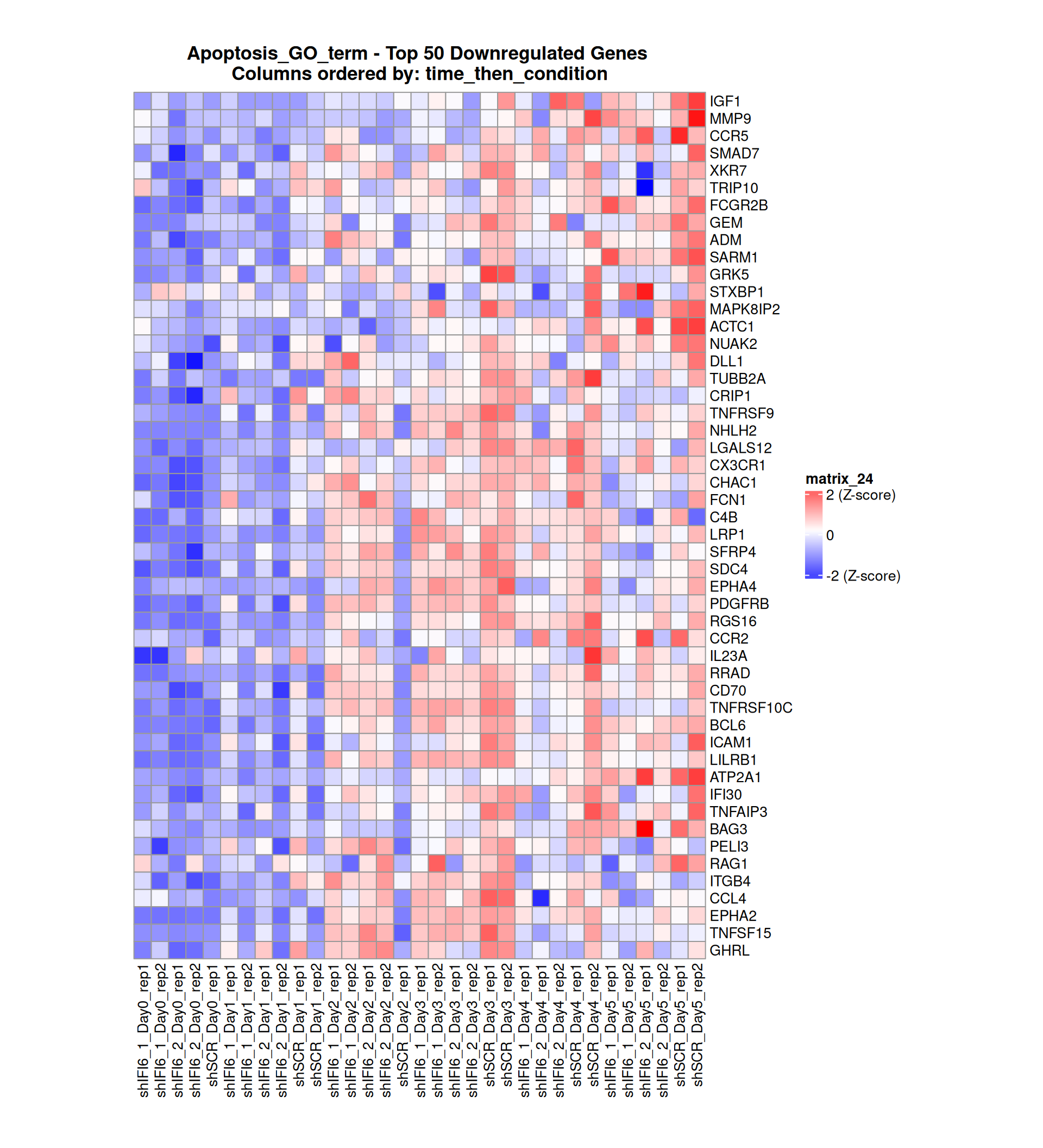
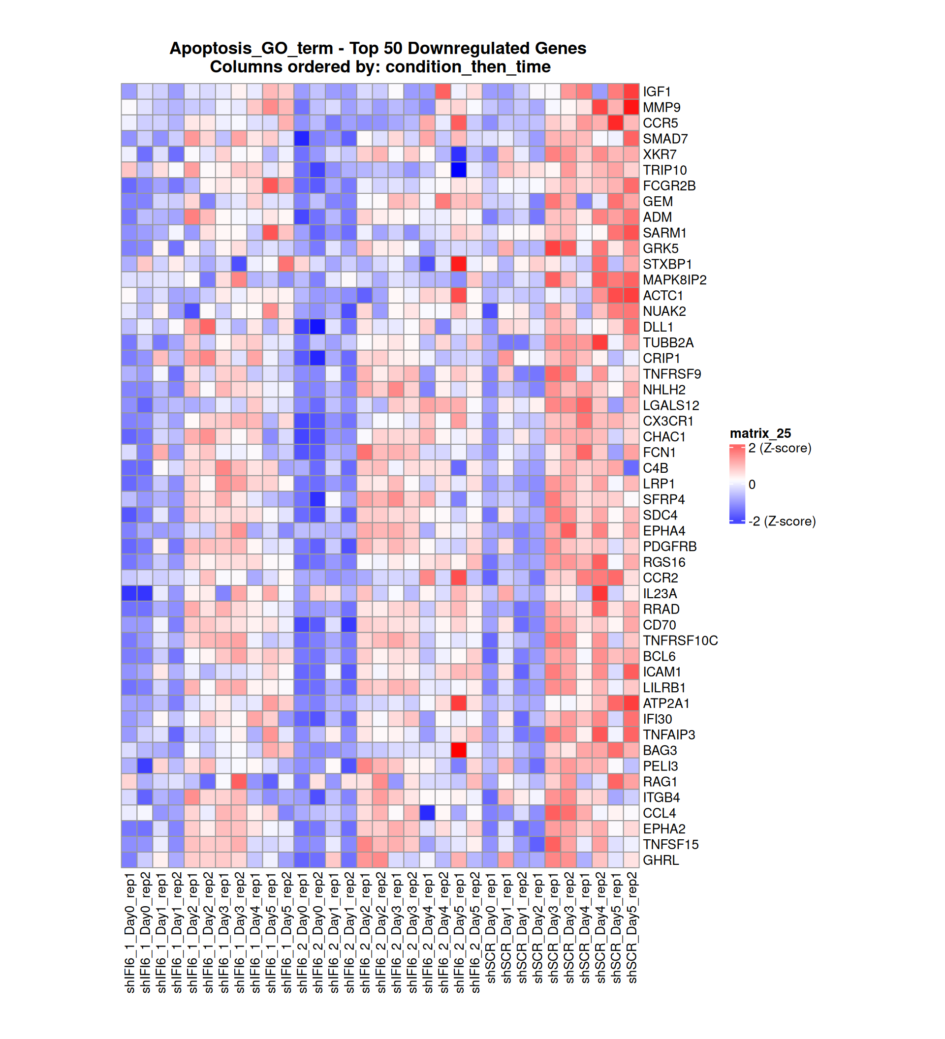
Gene expression Heatmaps
Below, we present some heatmaps depicting the expression levels of the selected set of genes, filtered to include only those identified as differentially expressed (DEGs). Consequently, the heatmap features genes from the selected list that overlap with the DEG subset. Accompanying the heatmap is a table summarizing the differential expression analysis results for these genes. Each gene is represented by multiple rows in the table, corresponding to the number of comparisons conducted.
The genes in the heatmaps are ordered specifically to highlight the differential expression between the two considered conditions: shIFI6 and shSCR. This is accomplished by ordering the results of the differential gene expression between the two conditions by log2 fold change and:
taking the highest value if the log2 fold change is positive
taking the lowest value if the log2 fold change is negative
taking the average if the log2 fold change in the two cases is one negative and one positive
The length of the HALLMARK list of genes is: 590. Considering that the heatmaps list only the top 50 up- and downregulated genes, there are 490 genes not shown in the heatmaps.
The length of the Cytokine list of genes is: 265. Considering that the heatmaps list only the top 50 up- and downregulated genes, there are 165 genes not shown in the heatmaps.
The length of the Inflammation list of genes is: 379. Considering that the heatmaps list only the top 50 up- and downregulated genes, there are 279 genes not shown in the heatmaps.
The length of the Interferon list of genes is: 40. Since there are fewer than 50 genes, all of them are shown in the heatmap.
The length of the Apoptosis list of genes is: 454. Considering that the heatmaps list only the top 50 up- and downregulated genes, there are 354 genes not shown in the heatmaps.
| Version | Author | Date |
|---|---|---|
| 078db00 | Mariani_Gianluca_Alessio | 2025-10-20 |
| Version | Author | Date |
|---|---|---|
| 078db00 | Mariani_Gianluca_Alessio | 2025-10-20 |
| Version | Author | Date |
|---|---|---|
| 078db00 | Mariani_Gianluca_Alessio | 2025-10-20 |
| Version | Author | Date |
|---|---|---|
| 078db00 | Mariani_Gianluca_Alessio | 2025-10-20 |
| Version | Author | Date |
|---|---|---|
| 078db00 | Mariani_Gianluca_Alessio | 2025-10-20 |
| Version | Author | Date |
|---|---|---|
| 078db00 | Mariani_Gianluca_Alessio | 2025-10-20 |
Gene expression Heatmap
ongoing
Library Sizes
A bar plot displaying total read counts per sample is shown below
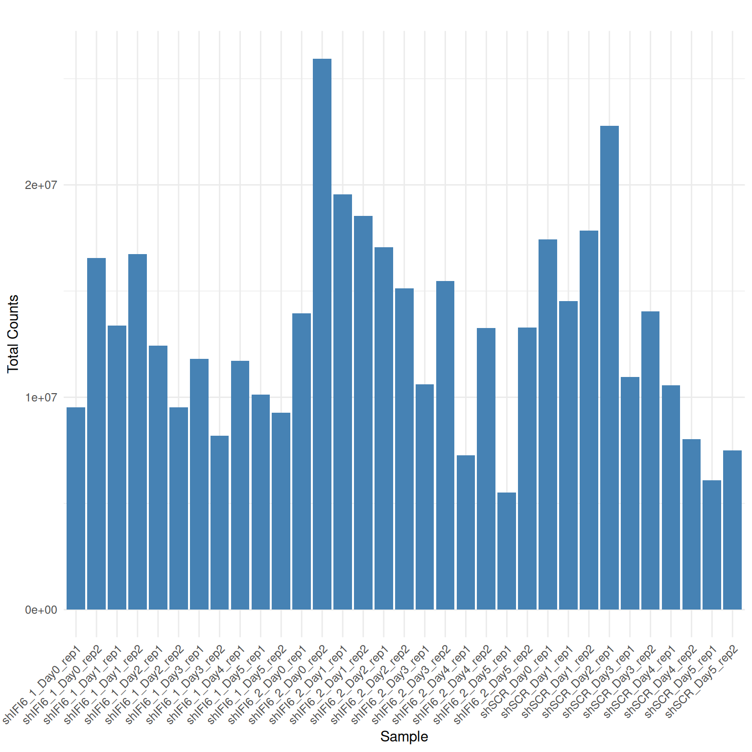
Interpretation Library Sizes
Variable but not extremely variable
Violin plot of VST-normalized counts
Below we present a violin plot of the VST-normalized read counts by sample.
A violin plot of VST-normalized counts provides an overview of the global distribution of gene expression values across samples after normalization. This plot allows for the detection of potential outliers, technical biases, or inconsistencies in distribution across samples, which could affect downstream analyses. A consistent distribution of VST counts across samples suggests successful normalization and comparable expression profiles.
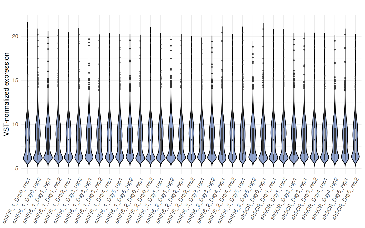
Interpretation Violin plot of VST-normalized counts
The violin plot of counts data displays a consistent distribution of
VST counts across samples.
This indicates no substantial differences in gene expression profiles
between the conditions and confirms the quality and reliability of the
samples, supporting the inclusion of all samples in subsequent
analyses.
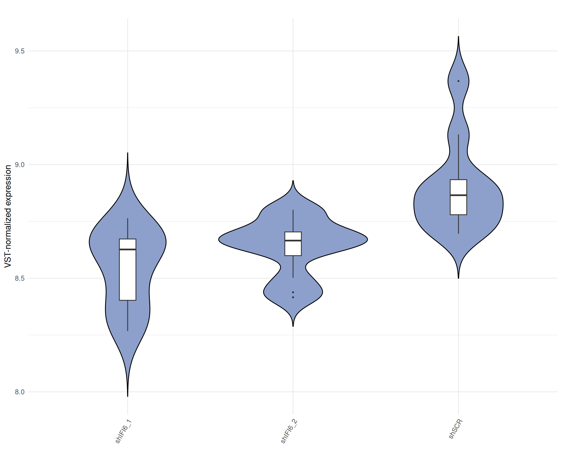
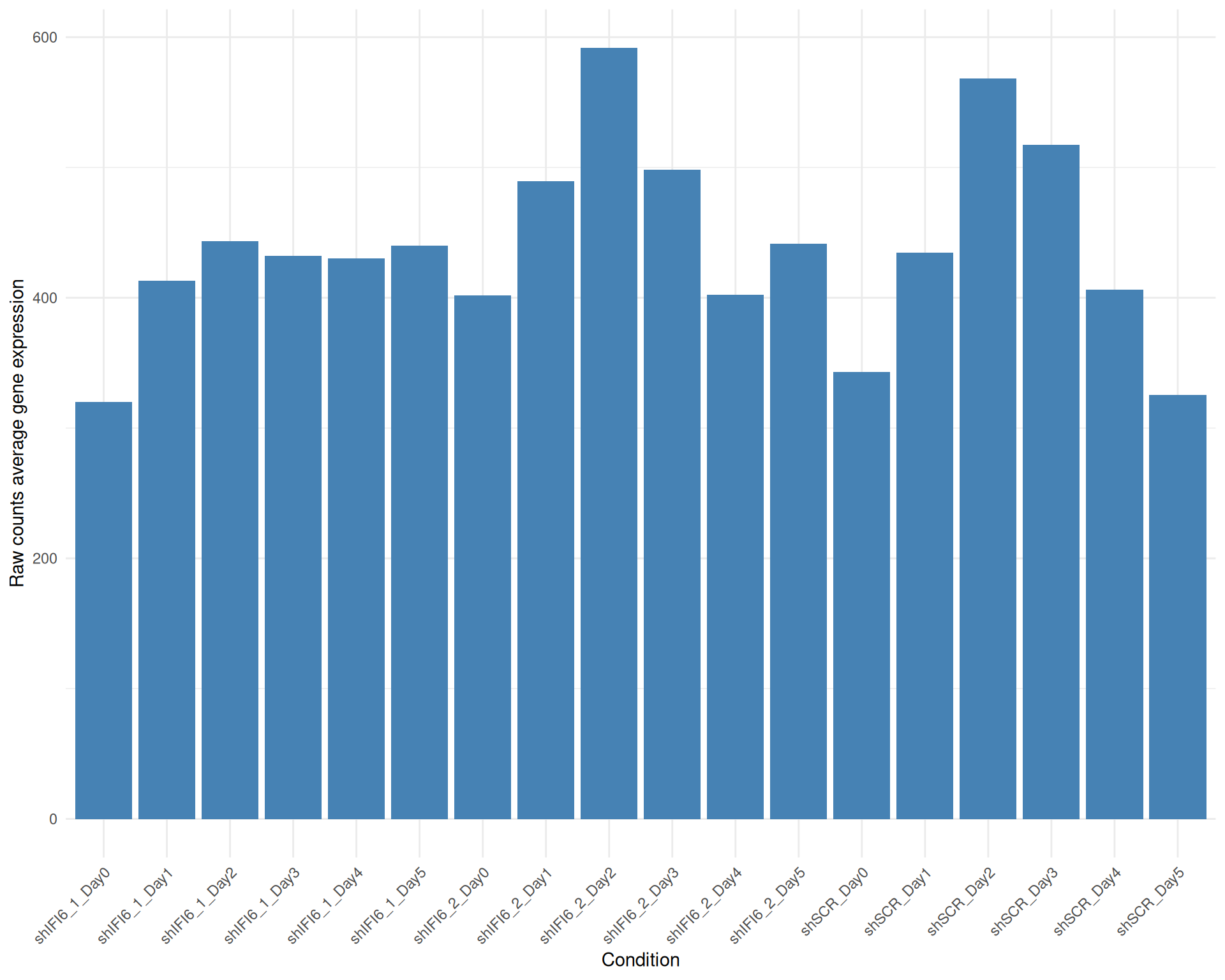
Average Expression across all samples
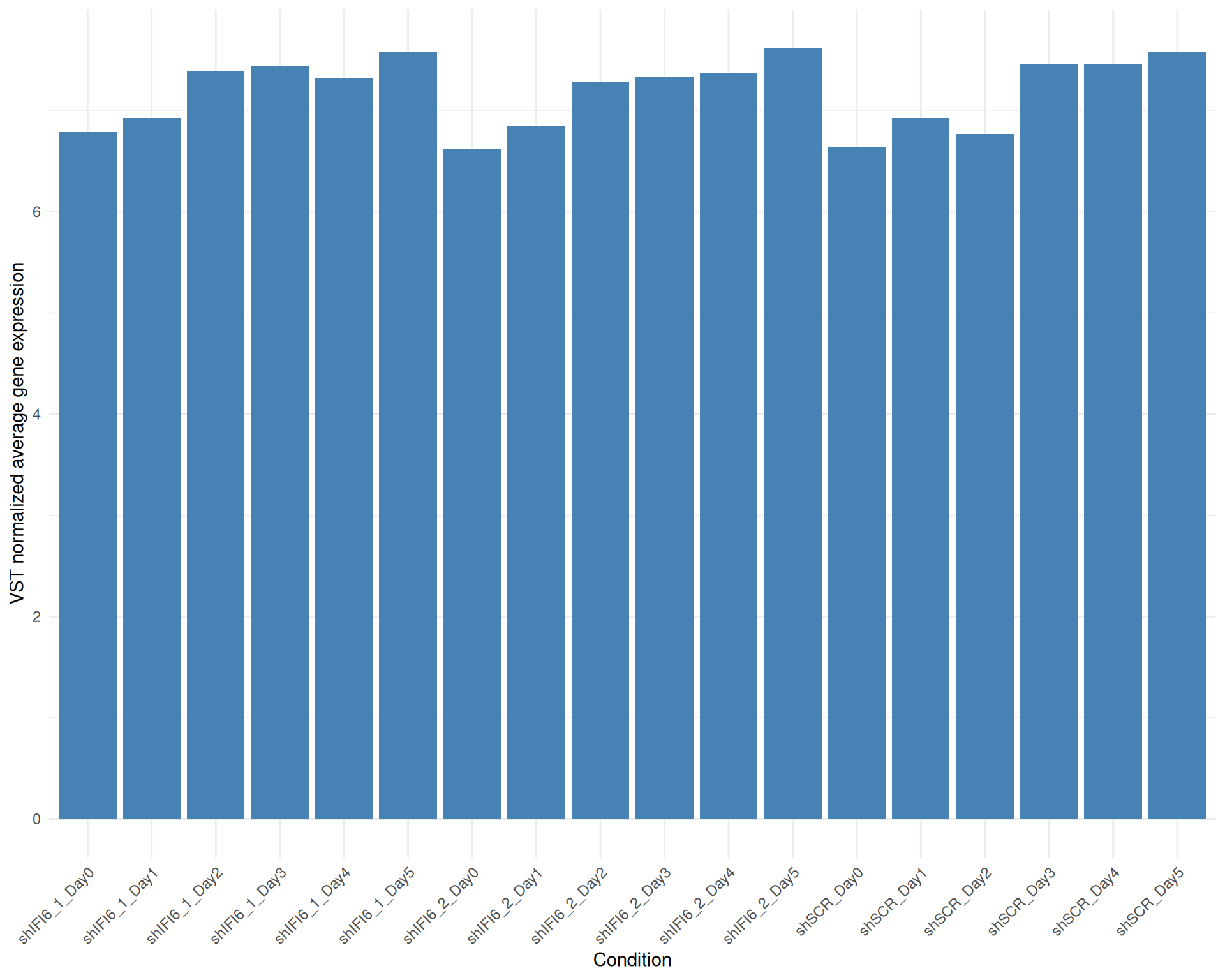
Below we present the distributions of the selected genes expression across conditions in a barplot where the height of each bar represents the average expression of all the selected genes in that particular condition. Each condition includes all the available replicates except those already filtered.
Average Expression, Raw counts, gene list: 251015_genelist_frascolla.csv
| Version | Author | Date |
|---|---|---|
| 078db00 | Mariani_Gianluca_Alessio | 2025-10-20 |
Average Expression, VST normalized counts, gene list: 251015_genelist_frascolla.csv
| Version | Author | Date |
|---|---|---|
| 078db00 | Mariani_Gianluca_Alessio | 2025-10-20 |
R version 4.5.0 (2025-04-11)
Platform: x86_64-pc-linux-gnu
Running under: Ubuntu 24.04.2 LTS

Matrix products: default
BLAS:   /usr/lib/x86_64-linux-gnu/openblas-pthread/libblas.so.3
LAPACK: /usr/lib/x86_64-linux-gnu/openblas-pthread/libopenblasp-r0.3.26.so;  LAPACK version 3.12.0

locale:
 [1] LC_CTYPE=en_US.UTF-8       LC_NUMERIC=C
 [3] LC_TIME=en_US.UTF-8        LC_COLLATE=en_US.UTF-8
 [5] LC_MONETARY=en_US.UTF-8    LC_MESSAGES=en_US.UTF-8
 [7] LC_PAPER=en_US.UTF-8       LC_NAME=C
 [9] LC_ADDRESS=C               LC_TELEPHONE=C
[11] LC_MEASUREMENT=en_US.UTF-8 LC_IDENTIFICATION=C

time zone: Etc/UTC
tzcode source: system (glibc)

attached base packages:
[1] stats4    grid      stats     graphics  grDevices utils     datasets
[8] methods   base

other attached packages:
 [1] ReactomePA_1.53.0           msigdbr_25.1.1
 [3] org.Hs.eg.db_3.21.0         AnnotationDbi_1.70.0
 [5] tibble_3.3.0                limma_3.64.3
 [7] gridExtra_2.3               WGCNA_1.73
 [9] fastcluster_1.3.0           dynamicTreeCut_1.63-1
[11] tidyr_1.3.1                 dplyr_1.1.4
[13] clusterProfiler_4.16.0      reshape_0.8.10
[15] gplots_3.2.0                RColorBrewer_1.1-3
[17] rtracklayer_1.68.0          DESeq2_1.48.2
[19] SummarizedExperiment_1.38.1 Biobase_2.68.0
[21] MatrixGenerics_1.20.0       matrixStats_1.5.0
[23] GenomicRanges_1.60.0        GenomeInfoDb_1.44.3
[25] IRanges_2.42.0              S4Vectors_0.46.0
[27] BiocGenerics_0.54.0         generics_0.1.4
[29] glue_1.8.0                  stringr_1.5.2
[31] reshape2_1.4.4              git2r_0.36.2
[33] DT_0.34.0                   ComplexHeatmap_2.24.1
[35] plotly_4.11.0               ggplot2_4.0.0

loaded via a namespace (and not attached):
  [1] splines_4.5.0            later_1.4.4              BiocIO_1.18.0
  [4] bitops_1.0-9             ggplotify_0.1.3          R.oo_1.27.1
  [7] polyclip_1.10-7          preprocessCore_1.70.0    graph_1.87.0
 [10] rpart_4.1.24             XML_3.99-0.19            lifecycle_1.0.4
 [13] doParallel_1.0.17        rprojroot_2.1.1          MASS_7.3-65
 [16] lattice_0.22-7           crosstalk_1.2.2          backports_1.5.0
 [19] magrittr_2.0.4           Hmisc_5.2-3              sass_0.4.10
 [22] rmarkdown_2.30           jquerylib_0.1.4          yaml_2.3.10
 [25] httpuv_1.6.16            ggtangle_0.0.7           cowplot_1.2.0
 [28] DBI_1.2.3                abind_1.4-8              purrr_1.1.0
 [31] R.utils_2.13.0           ggraph_2.2.2             RCurl_1.98-1.17
 [34] yulab.utils_0.2.1        nnet_7.3-20              tweenr_2.0.3
 [37] rappdirs_0.3.3           circlize_0.4.16          GenomeInfoDbData_1.2.14
 [40] enrichplot_1.28.4        ggrepel_0.9.6            tidytree_0.4.6
 [43] reactome.db_1.92.0       codetools_0.2-20         DelayedArray_0.34.1
 [46] ggforce_0.5.0            DOSE_4.2.0               tidyselect_1.2.1
 [49] shape_1.4.6.1            aplot_0.2.9              UCSC.utils_1.4.0
 [52] farver_2.1.2             viridis_0.6.5            base64enc_0.1-3
 [55] GenomicAlignments_1.44.0 jsonlite_2.0.0           GetoptLong_1.0.5
 [58] tidygraph_1.3.1          Formula_1.2-5            survival_3.8-3
 [61] iterators_1.0.14         foreach_1.5.2            tools_4.5.0
 [64] treeio_1.32.0            Rcpp_1.1.0               SparseArray_1.8.1
 [67] xfun_0.53                qvalue_2.40.0            withr_3.0.2
 [70] fastmap_1.2.0            caTools_1.18.3           digest_0.6.37
 [73] R6_2.6.1                 gridGraphics_0.5-1       colorspace_2.1-2
 [76] Cairo_1.6-5              GO.db_3.21.0             gtools_3.9.5
 [79] dichromat_2.0-0.1        RSQLite_2.4.3            R.methodsS3_1.8.2
 [82] data.table_1.17.8        graphlayouts_1.2.2       httr_1.4.7
 [85] htmlwidgets_1.6.4        S4Arrays_1.8.1           graphite_1.55.0
 [88] whisker_0.4.1            pkgconfig_2.0.3          gtable_0.3.6
 [91] blob_1.2.4               impute_1.82.0            workflowr_1.7.2
 [94] S7_0.2.0                 XVector_0.48.0           htmltools_0.5.8.1
 [97] fgsea_1.34.2             clue_0.3-66              scales_1.4.0
[100] png_0.1-8                ggfun_0.2.0              knitr_1.50
[103] rstudioapi_0.17.1        rjson_0.2.23             checkmate_2.3.3
[106] nlme_3.1-168             curl_7.0.0               cachem_1.1.0
[109] GlobalOptions_0.1.2      KernSmooth_2.23-26       parallel_4.5.0
[112] foreign_0.8-90           restfulr_0.0.16          pillar_1.11.1
[115] vctrs_0.6.5              promises_1.3.3           cluster_2.1.8.1
[118] htmlTable_2.4.3          evaluate_1.0.5           magick_2.9.0
[121] cli_3.6.5                locfit_1.5-9.12          compiler_4.5.0
[124] Rsamtools_2.24.1         rlang_1.1.6              crayon_1.5.3
[127] labeling_0.4.3           plyr_1.8.9               fs_1.6.6
[130] stringi_1.8.7            viridisLite_0.4.2        BiocParallel_1.42.2
[133] babelgene_22.9           assertthat_0.2.1         Biostrings_2.76.0
[136] lazyeval_0.2.2           GOSemSim_2.34.0          Matrix_1.7-4
[139] patchwork_1.3.2          bit64_4.6.0-1            statmod_1.5.0
[142] KEGGREST_1.48.1          igraph_2.1.4             memoise_2.0.1
[145] bslib_0.9.0              ggtree_3.16.3            fastmatch_1.1-6
[148] bit_4.6.0                ape_5.8-1                gson_0.1.0