Last updated: 2025-09-29
Checks: 7 0
Knit directory: frascolla_chemoresistance/
This reproducible R Markdown analysis was created with workflowr (version 1.7.2). The Checks tab describes the reproducibility checks that were applied when the results were created. The Past versions tab lists the development history.
Great! Since the R Markdown file has been committed to the Git repository, you know the exact version of the code that produced these results.
Great job! The global environment was empty. Objects defined in the global environment can affect the analysis in your R Markdown file in unknown ways. For reproduciblity it’s best to always run the code in an empty environment.
The command set.seed(20250522) was run prior to running
the code in the R Markdown file. Setting a seed ensures that any results
that rely on randomness, e.g. subsampling or permutations, are
reproducible.
Great job! Recording the operating system, R version, and package versions is critical for reproducibility.
Nice! There were no cached chunks for this analysis, so you can be confident that you successfully produced the results during this run.
Great job! Using relative paths to the files within your workflowr project makes it easier to run your code on other machines.
Great! You are using Git for version control. Tracking code development and connecting the code version to the results is critical for reproducibility.
The results in this page were generated with repository version 52502b5. See the Past versions tab to see a history of the changes made to the R Markdown and HTML files.
Note that you need to be careful to ensure that all relevant files for
the analysis have been committed to Git prior to generating the results
(you can use wflow_publish or
wflow_git_commit). workflowr only checks the R Markdown
file, but you know if there are other scripts or data files that it
depends on. Below is the status of the Git repository when the results
were generated:
Untracked files:
Untracked: .DS_Store
Untracked: analysis/_expression_barplot.Rmd
Untracked: data/RNAseq_analysis.xlsx
Untracked: data/RNAseq_analysis_gene_lists.xlsx
Untracked: data/UNIQUELIST_shIFI6_vs_shIFI6.csv
Untracked: data/UNIQUELIST_shIFI6_vs_shSCR.csv
Untracked: data/samples_info_sh1plus2_vs_scr.tsv
Untracked: data/shIFI6 Day 5 vs Day 0.csv
Untracked: data/shIFI6Day 3 vs shSCRDay 0.csv
Untracked: data/shIFI6Day 4 vs Day 0.csv
Untracked: data/shIFI6Day 4 vs shSCRDay 0.csv
Untracked: data/shIFI6Day 5 vs shSCRDay 0.csv
Untracked: data/shIFI6Day3 vs Day0.csv
Untracked: output/deg_shIFI6_Day0_vs_shSCR_Day0.tsv
Untracked: output/deg_shIFI6_Day1_vs_shSCR_Day0.tsv
Untracked: output/deg_shIFI6_Day2_vs_shSCR_Day0.tsv
Untracked: output/deg_shIFI6_Day3_vs_shSCR_Day0.tsv
Untracked: output/deg_shIFI6_Day4_vs_shSCR_Day0.tsv
Untracked: output/deg_shIFI6_Day5_vs_shSCR_Day0.tsv
Untracked: output/deg_shSCR_Day2_vs_shSCR_Day0.tsv
Untracked: output/deg_shSCR_Day3_vs_shSCR_Day0.tsv
Untracked: output/deg_shSCR_Day4_vs_shSCR_Day0.tsv
Untracked: src/a
Untracked: src/genes2filter_ensemblid.csv
Untracked: src/genes2filter_symbol.csv
Untracked: src/h.all.v2025.1.Hs.symbols.gmt
Unstaged changes:
Modified: output/deg_shIFI6_1_Day1_vs_shSCR_Day1.tsv
Modified: output/deg_shIFI6_1_Day2_vs_shSCR_Day2.tsv
Modified: output/deg_shIFI6_1_Day3_vs_shSCR_Day3.tsv
Modified: output/deg_shIFI6_1_Day4_vs_shSCR_Day4.tsv
Modified: output/deg_shIFI6_1_Day5_vs_shSCR_Day5.tsv
Modified: output/deg_shIFI6_2_Day1_vs_shSCR_Day1.tsv
Modified: output/deg_shIFI6_2_Day2_vs_shSCR_Day2.tsv
Modified: output/deg_shIFI6_2_Day3_vs_shSCR_Day3.tsv
Modified: output/deg_shIFI6_2_Day4_vs_shSCR_Day4.tsv
Modified: output/deg_shIFI6_2_Day5_vs_shSCR_Day5.tsv
Modified: output/deg_shIFI6_Day1_vs_shIFI6_Day0.tsv
Modified: output/deg_shIFI6_Day1_vs_shSCR_Day1.tsv
Modified: output/deg_shIFI6_Day2_vs_shIFI6_Day0.tsv
Modified: output/deg_shIFI6_Day2_vs_shSCR_Day2.tsv
Modified: output/deg_shIFI6_Day3_vs_shIFI6_Day0.tsv
Modified: output/deg_shIFI6_Day3_vs_shSCR_Day3.tsv
Modified: output/deg_shIFI6_Day4_vs_shIFI6_Day0.tsv
Modified: output/deg_shIFI6_Day4_vs_shSCR_Day4.tsv
Modified: output/deg_shIFI6_Day5_vs_shIFI6_Day0.tsv
Modified: output/deg_shIFI6_Day5_vs_shSCR_Day5.tsv
Modified: output/deg_shSCR_Day1_vs_shSCR_Day0.tsv
Modified: output/deg_shSCR_Day5_vs_shSCR_Day0.tsv
Modified: src/__utils_rna_seq_functions.R
Note that any generated files, e.g. HTML, png, CSS, etc., are not included in this status report because it is ok for generated content to have uncommitted changes.
These are the previous versions of the repository in which changes were
made to the R Markdown (analysis/04_de_ifi6_day5_day0.Rmd)
and HTML (docs/04_de_ifi6_day5_day0.html) files. If you’ve
configured a remote Git repository (see ?wflow_git_remote),
click on the hyperlinks in the table below to view the files as they
were in that past version.
| File | Version | Author | Date | Message |
|---|---|---|---|---|
| Rmd | 52502b5 | Mariani_Gianluca_Alessio | 2025-09-29 | Added enrichment score for every pathway in the GSEA, added GO and HALLMARK terms for every gene in the genetables |
| html | 11f3d4d | Mariani_Gianluca_Alessio | 2025-07-16 | Build site. |
| Rmd | 4110172 | Mariani_Gianluca_Alessio | 2025-07-16 | Redone analysis with HALLMARK GSEA and fixed goenrichment ORA function with check to stop if genelist empty after various filters inside goenrichment function |
| html | 401e86f | Mariani_Gianluca_Alessio | 2025-07-15 | Build site. |
| Rmd | 57ef6f7 | Mariani_Gianluca_Alessio | 2025-07-15 | Redone analysis with ribosomal genes filter |
| html | fea3f82 | Yinxiu Zhan | 2025-07-11 | Build site. |
| html | 3839c7f | Yinxiu Zhan | 2025-07-10 | Build site. |
| Rmd | 4b13018 | Yinxiu Zhan | 2025-07-10 | Add all reports |
| Rmd | c0a0612 | Yinxiu Zhan | 2025-07-09 | :sparkles: Release first version |
knitr::opts_chunk$set(echo = FALSE,
message = FALSE,
warning = FALSE,
cache = FALSE,
autodep = TRUE,
fig.align = 'center',
fig.width = 10,
fig.height = 8)shIFI6_Day5 vs shIFI6_Day0
The objective of this report is to investigate differential gene expression between the two conditions and to conduct gene ontology enrichment analysis to explore the biological functions involved.
Parameters
Below is the list of parameters used in this report to define differential gene expression.
- logfc = 1
- qvalue = 0.05 , Adjusted p-value threshold (false discovery rate)
- Lowly expressed genes are removed to reduce noise. Lowly expressed
genes are here considered as:
- genes having total number of reads less than half of the total samples, 16 ;
- genes expressed in less samples than the total number of conditions,
12 .
Comparison Group and Differential Gene Expression Analysis Plan
Below we show the comparison group considered for the analysis presented in this report. Each group contains all the samples associated to the specific condition we want to conduct the analysis on.
The group is divided into experimental samples and control samples.
Each differential gene expression comparison will be conducted between these two groups.
Group considered:
- Experimental samples
(shIFI6_Day5):
shIFI6_1_Day5_rep1
shIFI6_1_Day5_rep2
shIFI6_2_Day5_rep1
shIFI6_2_Day5_rep2
-
Control Samples
(shIFI6_Day0):
shIFI6_1_Day0_rep1
shIFI6_1_Day0_rep2
shIFI6_2_Day0_rep1
shIFI6_2_Day0_rep2
The RNAseq data for this analysis:
- aim to investigate what is the difference in gene expression between shIFI6_Day5 and shIFI6_Day0
The sample population include:
- 23 samples, 2 conditions, shIFI6_Day5 and shIFI6_Day0 in 2 replicates each.
PCA
Below we present the PCA analysis conducted on the two specific conditions analyzed in this report.
Interpretation PCA Analysis
Missing Interpretation
MA plot and volcano plot
MA plot
The MA plot is a widely used visualization in differential expression analysis that displays the relationship between the average expression (A) and the log fold change (M) for each gene. The x-axis represents the mean expression level across samples, while the y-axis shows the log fold change between groups.
Total number of significant genes: 2314
Volcano plot
The Volcano plot is a graphical method to visualize differential expression results by combining statistical significance and magnitude of change for each gene. It plots the log2 fold change on the x-axis against the negative log10 of the p-value (or adjusted p-value) on the y-axis.
Tables of genes
Below we present two tables, the first includes all the genes identified in the analysis while the second includes only the differentially expressed genes (DEG)
Table of all genes
The columns in the table are:
baseMean: The average normalized count of a gene across all samples, reflecting its overall expression level in the dataset.
log2FoldChange: The estimated log2-transformed fold change in expression between two conditions (experimental vs control). Positive values indicate upregulation, negative values indicate downregulation with respect to control.
lfcSE: The standard error associated with the log2 fold change estimate, indicating the variability or uncertainty of the fold change measurement.
stat: The test statistic value calculated for the hypothesis test of whether the log2 fold change differs from zero.
pvalue: The raw p-value corresponding to the statistical test for differential expression; it reflects the probability of observing the data assuming no true difference in expression.
padj: The p-value adjusted for multiple testing (using the Benjamini-Hochberg method) to control the false discovery rate (FDR), providing a more reliable significance measure.
comparison_exp_vs_contr: A label or descriptor indicating the comparison made, specifying which condition is experimental and which is control.
gene: The unique Ensembl identifier for each gene as annotated in the reference genome.
symbol: The gene symbol or common gene name, which is easier to interpret biologically than numerical IDs.
FoldChange: The fold change in linear scale (non-logarithmic), derived from log2FoldChange (i.e., 2^(log2FoldChange)), representing how many times expression has changed.
differentially_expressed: A categorical variable indicating whether the gene is considered differentially expressed (“yes” or “no”) based on the predefined thresholds for significance and fold change described in the next section.
Table of differentially expressed genes
In this table we can find a subset of the previous table that includes the differentially expressed genes (DEGs).
The genes defined as DEGs need to satisfy these two conditions:
- The associated padj (p-value adjusted for multiple testing) must be inferior to the qvalue of 0.05 ;
- The associated log2FoldChange absolute value must be superior to the
logfc value of 1 .
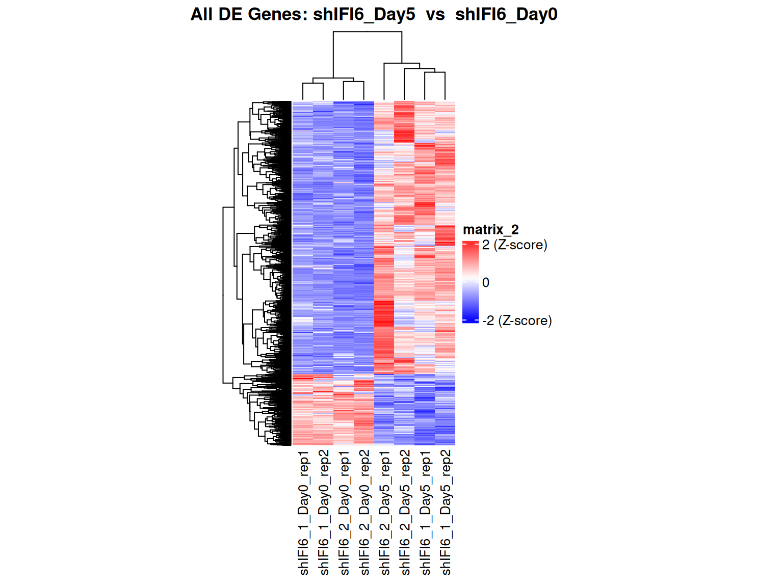
Heatmaps
Given the significant genes, among the differentially expressed genes previously computed, below a visualization of all the DE genes.
Meaning of Colors
- Red: Indicates high expression for that gene in a given sample (value above average, positive compared to the standardized scale).
- Blue: Indicates low expression for that gene in a given sample (value below average, negative compared to the standardized scale).
- White (or intermediate color): Indicates an expression close to the average (standardized value around 0).
Heatmap for all genes
This heatmap displays the expression levels of all genes detected in the RNA-seq dataset across all samples. The values are normalized and transformed (via variance stabilizing transformation) to allow comparison across genes and samples. This comprehensive visualization provides an overview of the global expression patterns, highlighting overall similarities and differences between samples, as well as potential outliers.
Gene set enrichment analysis
Further analysis is done through gene set enrichment analysis, which does not exclude genes based on logfc or adjusted p-value, as done previously.
GSEA - GO
GSEA is performed separately on each subontology: biological processes (BP), cellular components (CC) and molecular functions (MF). The dot plot below shows all the enriched GO terms. The size of each dot correlates with the count of differentially expressed genes associated with each GO term. Furthermore, the color of each dot reflects the significance of the enrichment of the respective GO term, highlighting its relative importance.
GO - Biological Processes
shIFI6_Day5 vs shIFI6_Day0
P value cutoff: 0.05
GO - Cellular Components
shIFI6_Day5 vs shIFI6_Day0
P value cutoff: 0.05
GSEA - Hallmark
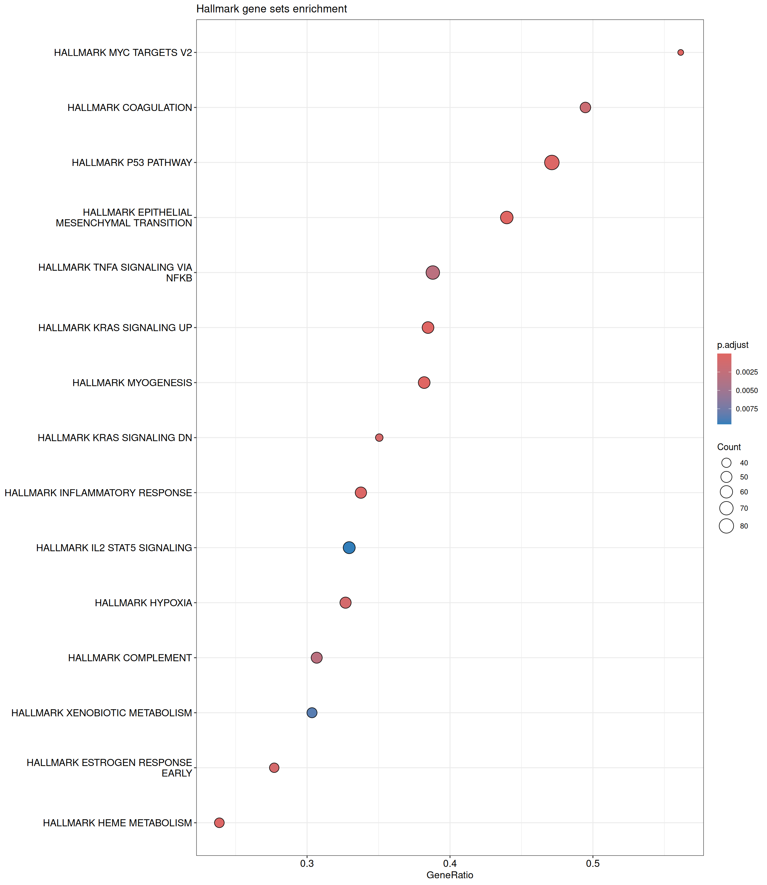
GSEA is performed using the Hallmark gene sets, which represent well-defined biological states and processes. The dot plot below displays all enriched Hallmark pathways. The size of each dot corresponds to the number of differentially expressed genes contributing to each pathway. Additionally, the color of each dot indicates the significance of the pathway’s enrichment, emphasizing its relative importance.
Hallmark Gene Sets
shIFI6_Day5 vs shIFI6_Day0
P value cutoff: 0.05
| Version | Author | Date |
|---|---|---|
| 11f3d4d | Mariani_Gianluca_Alessio | 2025-07-16 |
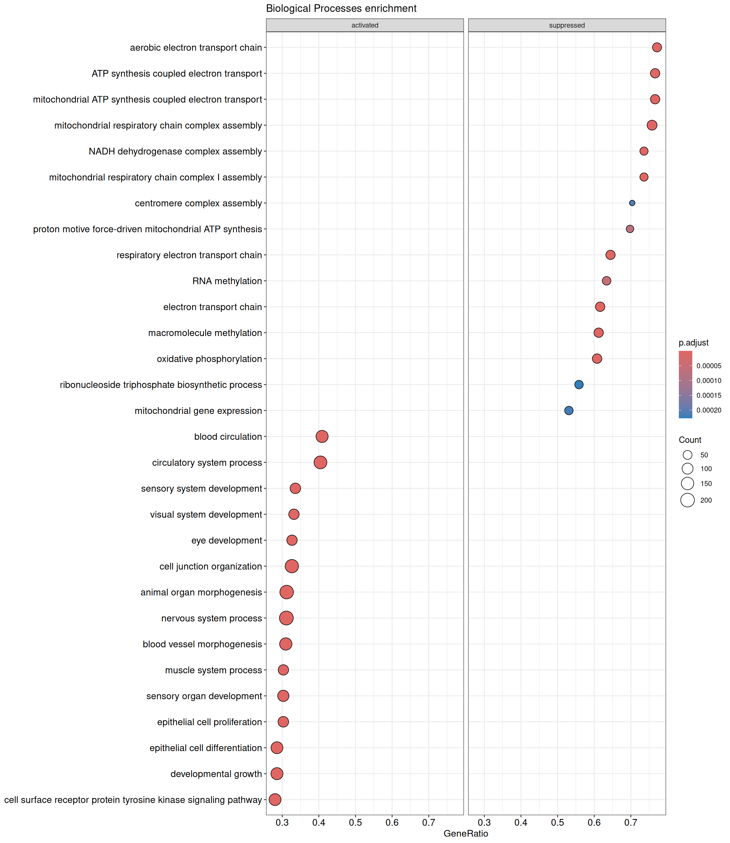
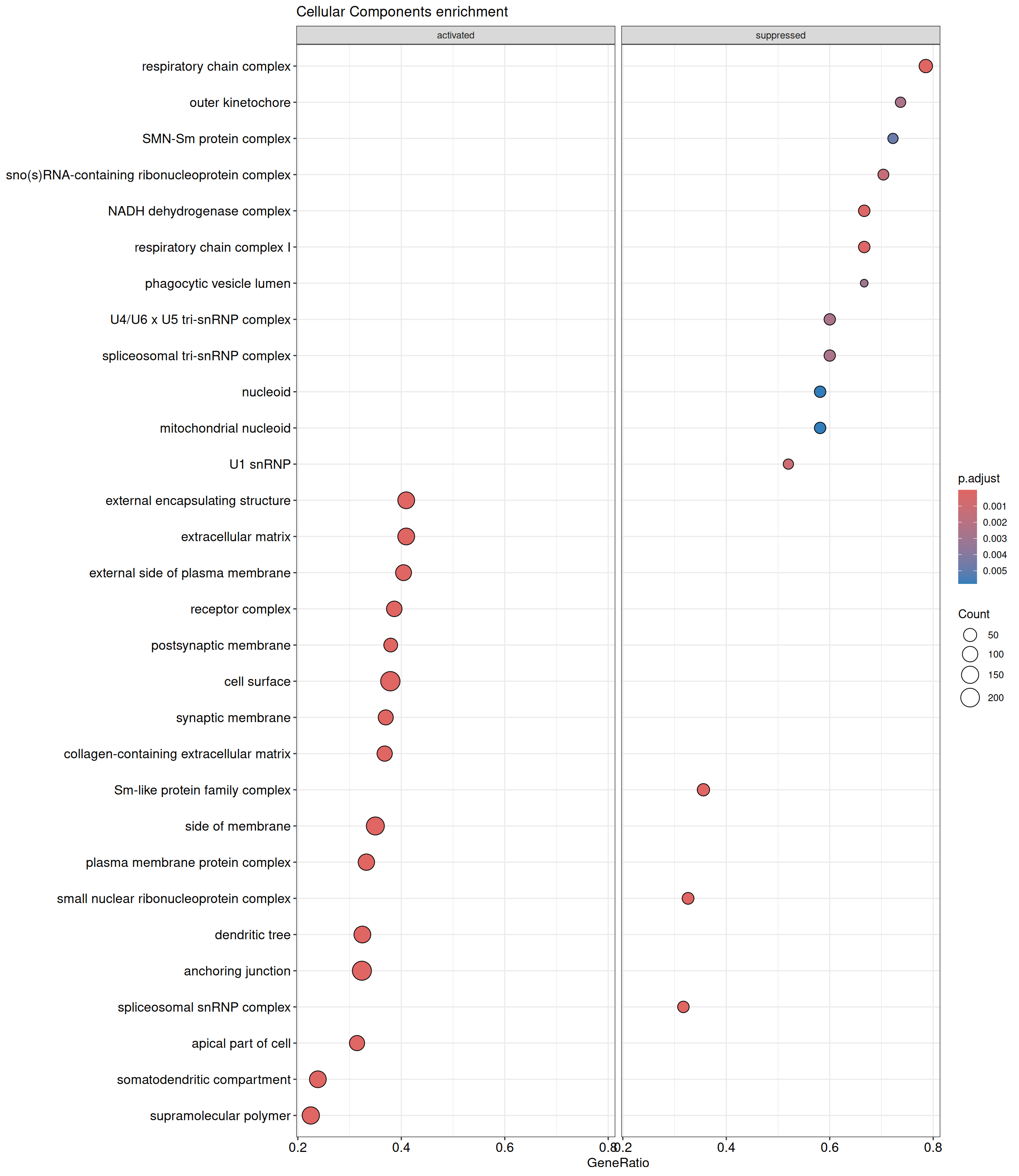
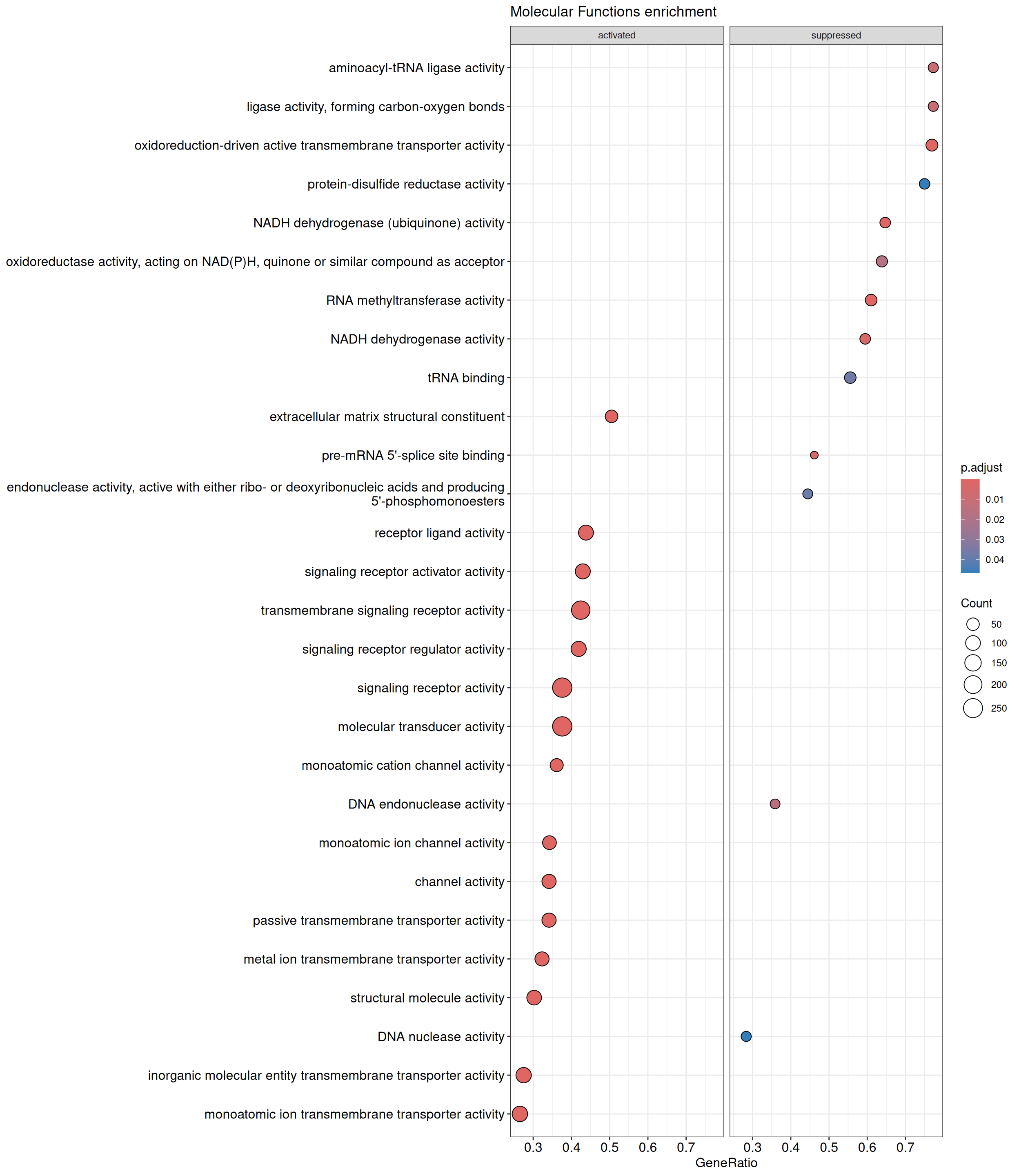
Over representation analysis
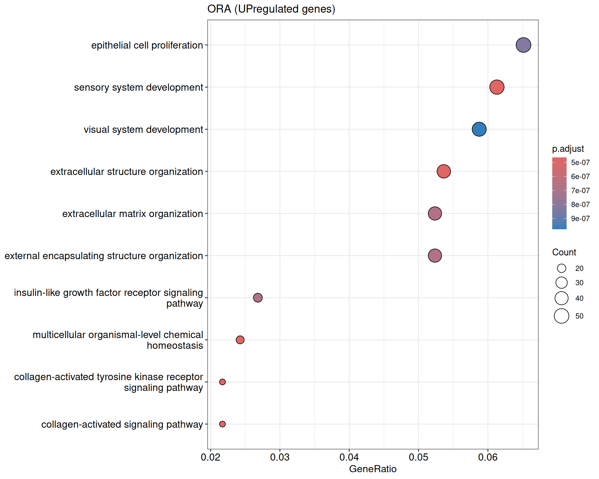
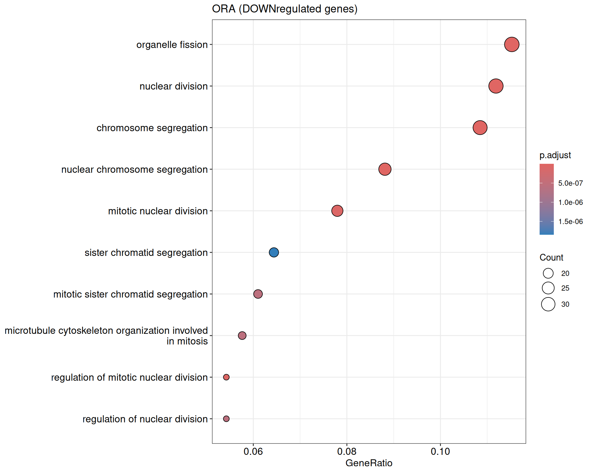
We performed a functional enrichment analysis based on Over-Representation Analysis (ORA) using the GO pathway database. Unlike GSEA, which considers the entire ranked list of genes, ORA focuses only on genes that meet specific differential expression thresholds (adjusted p-value and log2 fold change). The analysis was conducted separately for upregulated and downregulated genes to identify GO pathways that are significantly enriched in each group, compared to what would be expected by chance. This allows for a clearer biological interpretation of distinct transcriptional programs activated or suppressed in the dataset. The dot plots below display all significantly enriched GO pathways. Each dot’s size represents the number of differentially expressed genes associated with the pathway, while the color reflects the statistical significance of the enrichment (adjusted p-value).
The following genes are not valid symbols and will be removed from the analysis:
AC003102.3, AC005264.2, AC007551.3, AC007880.1, AC011747.4, AC020571.3, AC058791.1, AC074138.3, AC096559.1, AC147651.4, AF064858.7, AIM1L, AKAP2, ALG1L, AMICA1, ARNTL, BAALCOS, BAI2, BOLA3-AS1, BZRAP1, C10orf10, C12orf39, C12orf5, C12orf68, C12orf74, C14orf28, C15orf26, C15orf59, C17orf82, C19orf59, C1orf101, C1orf145, C1orf200, C20orf197, C2orf91, C3orf27, C3orf35, C3orf65, C3orf67, C5orf30, C5orf54, C6orf164, C9orf139, CASC14, CCBL1, CCDC173, CCDC19, CD97, CEBPA-AS1, CECR6, CIDECP, CLK2P, CSTF3-AS1, DKFZP434F142, DKFZp667F0711, EFCAB4A, ELMSAN1, EMR2, EMR4P, FAIM3, FAM129A, FAM154B, FAM173A, FAM183B, FAM189A1, FAM196A, FAM198A, FAM198B, FAM19A5, FAM211A, FAM212B, FAM212B-AS1, FAM213A, FAM214B, FAM26F, FAM46A, FAM46B, FAM46C, FAM57B, FAM64A, FAM65C, FAM71A, FCGR1B, FCGR1C, FKBP9L, FLG-AS1, FLJ26850, FLJ35934, FLJ42258, FLJ44342, GATS, GGTA1P, GK3P, GNN, GPR128, GPR98, H1F0, HCCAT4, HIST1H1B, HIST1H1C, HIST1H1D, HIST1H2AB, HIST1H2AD, HIST1H2AE, HIST1H2AG, HIST1H2AH, HIST1H2AI, HIST1H2AK, HIST1H2BC, HIST1H2BD, HIST1H2BF, HIST1H2BG, HIST1H2BL, HIST1H2BO, HIST1H3B, HIST1H3D, HIST1H3F, HIST1H3H, HIST1H3I, HIST1H3J, HIST1H4B, HIST1H4C, HIST1H4D, HIST1H4E, HIST1H4H, HIST1H4I, HIST1H4K, HIST1H4L, HIST2H2AA3, HIST2H2BC, HIST2H3C, HIST2H3D, HRASLS2, HRSP12, IGJ, KGFLP1, KIAA0226L, KIAA0355, KIAA1199, KIAA1462, KIAA1875, LARGE, LEPREL4, LINC00086, LINC00176, LINC00211, LINC00263, LINC00337, LINC00346, LINC00441, LINC00638, LINC00672, LINC00893, LINC01021, LOC100129518, LOC100129550, LOC100129940, LOC100130093, LOC100130520, LOC100130705, LOC100131825, LOC100132874, LOC100134822, LOC100287497, LOC100505761, LOC100506157, LOC100506351, LOC100506538, LOC100506691, LOC100506737, LOC100507156, LOC100507191, LOC100507258, LOC100507460, LOC100507487, LOC100507642, LOC100652901, LOC100653005, LOC100996273, LOC100996274, LOC100996442, LOC100996455, LOC100996570, LOC100996634, LOC100996761, LOC101059949, LOC101060181, LOC101060494, LOC101926967, LOC101927002, LOC101927063, LOC101927255, LOC101927407, LOC101927810, LOC101927850, LOC101927858, LOC101927910, LOC101927931, LOC101927943, LOC101928042, LOC101928054, LOC101928061, LOC101928072, LOC101928092, LOC101928113, LOC101928123, LOC101928186, LOC101928192, LOC101928360, LOC101928399, LOC101928429, LOC101928465, LOC101928482, LOC101928676, LOC101928722, LOC101928814, LOC101928841, LOC101929054, LOC101929191, LOC101929243, LOC101929295, LOC101929340, LOC101929346, LOC101929379, LOC101929580, LOC101929670, LOC102606465, LOC102723365, LOC102723455, LOC102723569, LOC102723587, LOC102723647, LOC102723648, LOC102723652, LOC102723843, LOC102723864, LOC102723902, LOC102723953, LOC102723972, LOC102724037, LOC102724164, LOC102724232, LOC102724238, LOC102724243, LOC102724258, LOC102724280, LOC102724296, LOC102724299, LOC102724312, LOC102724371, LOC102724516, LOC102724554, LOC102724571, LOC102724583, LOC102724634, LOC102724681, LOC102724740, LOC102724757, LOC102724788, LOC102724811, LOC102724814, LOC102724852, LOC102724854, LOC102724884, LOC102724944, LOC102724951, LOC102724967, LOC220729, LOC257358, LOC284561, LOC388210, LOC388780, LOC390937, LOC644794, LOC728613, LOC729222, LOC90834, LPPR2, LRRC16A, MARC1, MARC2, MARCH1, MARCH2, MARCH4, METTL12, METTL7B, MFSD4, MICALCL, MIR4697HG, MLLT4, MPP6, N6AMT2, NAPRT1, ODF3L1, PAPD5, PIFO, PPAPDC1A, PTCHD2, PVRL1, PVRL4, RGAG4, RNF144A-AS1, RP11-13A1.1, RP11-142C4.6, RP11-14J7.6, RP11-15A1.7, RP11-214C8.2, RP11-231I16.1, RP11-277P12.20, RP11-307C12.11, RP11-354E11.2, RP11-37B2.1, RP11-384K6.6, RP11-387D10.3, RP11-439L8.4, RP11-445H22.3, RP11-475N22.4, RP11-494M8.4, RP11-536C5.7, RP11-611D20.2, RP11-66B24.1, RP11-696N14.1, RP11-7F17.5, RP11-861A13.4, RP11-890B15.2, RP11-983P16.4, RP11-996F15.2, RP3-400B16.1, RP5-1033H22.2, RSG1, SDPR, SEPT4, SGOL2, SLC22A18AS, SLC9A3R2, SOGA2, SOGA3, ST3GAL4-AS1, ST5, TCTEX1D2, TCTEX1D4, TEPP, TMEM136, TRNE, WDR63, WDR66, XRCC6BP1, ZNF812
ORA - UP
shIFI6_Day5 vs shIFI6_Day0
P value cutoff: 0.05
Q value cutoff: 0.05
ORA - DOWN
shIFI6_Day5 vs shIFI6_Day0
P value cutoff: 0.05
Q value cutoff: 0.05
R version 4.5.0 (2025-04-11)
Platform: x86_64-pc-linux-gnu
Running under: Ubuntu 24.04.2 LTS
Matrix products: default
BLAS: /usr/lib/x86_64-linux-gnu/openblas-pthread/libblas.so.3
LAPACK: /usr/lib/x86_64-linux-gnu/openblas-pthread/libopenblasp-r0.3.26.so; LAPACK version 3.12.0
locale:
[1] LC_CTYPE=en_US.UTF-8 LC_NUMERIC=C
[3] LC_TIME=en_US.UTF-8 LC_COLLATE=en_US.UTF-8
[5] LC_MONETARY=en_US.UTF-8 LC_MESSAGES=en_US.UTF-8
[7] LC_PAPER=en_US.UTF-8 LC_NAME=C
[9] LC_ADDRESS=C LC_TELEPHONE=C
[11] LC_MEASUREMENT=en_US.UTF-8 LC_IDENTIFICATION=C
time zone: Etc/UTC
tzcode source: system (glibc)
attached base packages:
[1] stats4 grid stats graphics grDevices utils datasets
[8] methods base
other attached packages:
[1] msigdbr_25.1.1 ReactomePA_1.53.0
[3] tibble_3.3.0 limma_3.64.3
[5] org.Hs.eg.db_3.21.0 AnnotationDbi_1.70.0
[7] git2r_0.36.2 gridExtra_2.3
[9] WGCNA_1.73 fastcluster_1.3.0
[11] dynamicTreeCut_1.63-1 dplyr_1.1.4
[13] clusterProfiler_4.16.0 reshape_0.8.10
[15] DT_0.34.0 gplots_3.2.0
[17] RColorBrewer_1.1-3 rtracklayer_1.68.0
[19] DESeq2_1.48.2 SummarizedExperiment_1.38.1
[21] Biobase_2.68.0 MatrixGenerics_1.20.0
[23] matrixStats_1.5.0 GenomicRanges_1.60.0
[25] GenomeInfoDb_1.44.3 IRanges_2.42.0
[27] S4Vectors_0.46.0 BiocGenerics_0.54.0
[29] generics_0.1.4 ComplexHeatmap_2.24.1
[31] plotly_4.11.0 ggplot2_4.0.0
loaded via a namespace (and not attached):
[1] splines_4.5.0 later_1.4.4 BiocIO_1.18.0
[4] bitops_1.0-9 ggplotify_0.1.3 R.oo_1.27.1
[7] polyclip_1.10-7 preprocessCore_1.70.0 graph_1.87.0
[10] rpart_4.1.24 XML_3.99-0.19 lifecycle_1.0.4
[13] doParallel_1.0.17 rprojroot_2.1.1 MASS_7.3-65
[16] lattice_0.22-7 crosstalk_1.2.2 backports_1.5.0
[19] magrittr_2.0.4 Hmisc_5.2-3 sass_0.4.10
[22] rmarkdown_2.29 jquerylib_0.1.4 yaml_2.3.10
[25] httpuv_1.6.16 ggtangle_0.0.7 cowplot_1.2.0
[28] DBI_1.2.3 abind_1.4-8 purrr_1.1.0
[31] R.utils_2.13.0 ggraph_2.2.2 RCurl_1.98-1.17
[34] nnet_7.3-20 yulab.utils_0.2.1 tweenr_2.0.3
[37] rappdirs_0.3.3 circlize_0.4.16 GenomeInfoDbData_1.2.14
[40] enrichplot_1.28.4 ggrepel_0.9.6 tidytree_0.4.6
[43] reactome.db_1.92.0 codetools_0.2-20 DelayedArray_0.34.1
[46] ggforce_0.5.0 DOSE_4.2.0 tidyselect_1.2.1
[49] shape_1.4.6.1 aplot_0.2.9 UCSC.utils_1.4.0
[52] farver_2.1.2 viridis_0.6.5 base64enc_0.1-3
[55] GenomicAlignments_1.44.0 jsonlite_2.0.0 GetoptLong_1.0.5
[58] tidygraph_1.3.1 Formula_1.2-5 survival_3.8-3
[61] iterators_1.0.14 foreach_1.5.2 tools_4.5.0
[64] treeio_1.32.0 Rcpp_1.1.0 glue_1.8.0
[67] SparseArray_1.8.1 xfun_0.53 qvalue_2.40.0
[70] withr_3.0.2 fastmap_1.2.0 caTools_1.18.3
[73] digest_0.6.37 R6_2.6.1 gridGraphics_0.5-1
[76] colorspace_2.1-2 Cairo_1.6-5 GO.db_3.21.0
[79] gtools_3.9.5 dichromat_2.0-0.1 RSQLite_2.4.3
[82] R.methodsS3_1.8.2 tidyr_1.3.1 data.table_1.17.8
[85] graphlayouts_1.2.2 httr_1.4.7 htmlwidgets_1.6.4
[88] S4Arrays_1.8.1 graphite_1.55.0 whisker_0.4.1
[91] pkgconfig_2.0.3 gtable_0.3.6 blob_1.2.4
[94] impute_1.82.0 workflowr_1.7.2 S7_0.2.0
[97] XVector_0.48.0 htmltools_0.5.8.1 fgsea_1.34.2
[100] clue_0.3-66 scales_1.4.0 png_0.1-8
[103] ggfun_0.2.0 knitr_1.50 rstudioapi_0.17.1
[106] reshape2_1.4.4 rjson_0.2.23 checkmate_2.3.3
[109] nlme_3.1-168 curl_7.0.0 cachem_1.1.0
[112] GlobalOptions_0.1.2 stringr_1.5.2 KernSmooth_2.23-26
[115] parallel_4.5.0 foreign_0.8-90 restfulr_0.0.16
[118] pillar_1.11.1 vctrs_0.6.5 promises_1.3.3
[121] cluster_2.1.8.1 htmlTable_2.4.3 evaluate_1.0.5
[124] magick_2.9.0 cli_3.6.5 locfit_1.5-9.12
[127] compiler_4.5.0 Rsamtools_2.24.1 rlang_1.1.6
[130] crayon_1.5.3 labeling_0.4.3 plyr_1.8.9
[133] fs_1.6.6 stringi_1.8.7 viridisLite_0.4.2
[136] BiocParallel_1.42.2 babelgene_22.9 assertthat_0.2.1
[139] Biostrings_2.76.0 lazyeval_0.2.2 GOSemSim_2.34.0
[142] Matrix_1.7-4 patchwork_1.3.2 bit64_4.6.0-1
[145] statmod_1.5.0 KEGGREST_1.48.1 igraph_2.1.4
[148] memoise_2.0.1 bslib_0.9.0 ggtree_3.16.3
[151] fastmatch_1.1-6 bit_4.6.0 ape_5.8-1
[154] gson_0.1.0